00. Motivation

This tutorial provides the theoretical background for the methods used throughout the CaliBrain documentation. It introduces the forward model, the inverse uncertainty problem, empirical coverage, and post-hoc recalibration.

Why uncertainty calibration matters

CaliBrain addresses a methodological question in inverse source imaging: when a solver reports posterior uncertainty, does that uncertainty have the intended frequentist coverage under controlled simulation?

In the current documentation, this question is studied for posterior summaries produced by source estimation, transformed into uncertainty objects by uncertainty estimation, and then evaluated or recalibrated in calibration methods.

import matplotlib.pyplot as plt
import numpy as np

Forward model and inverse problem

In EEG/MEG source imaging, sensor measurements are modeled as

\[Y = L X + E,\]

where \(L\) is the leadfield, \(X\) is the unknown source activity, and \(E\) is sensor noise. The inverse problem is ill-posed because multiple source configurations can explain similar sensor patterns.

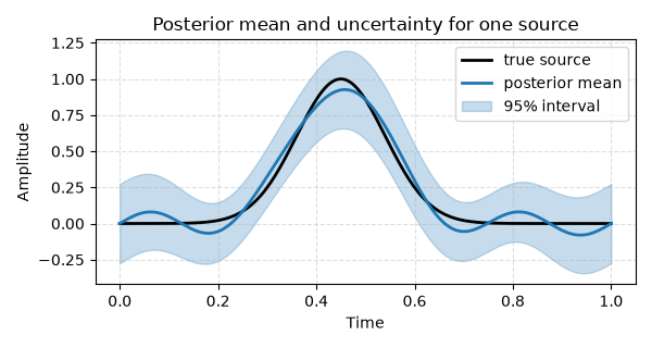
For that reason, CaliBrain treats inverse methods as posterior procedures: they should return not only a point estimate \(\hat{X}\), but also a posterior covariance or a reduced uncertainty representation derived from it.

The forward objects themselves are introduced in source simulation, leadfield construction, and sensor simulation.

time = np.linspace(0.0, 1.0, 200)
true_signal = np.exp(-0.5 * ((time - 0.45) / 0.09) ** 2)
posterior_mean = true_signal + 0.08 * np.sin(8 * np.pi * time)
posterior_std = 0.12 + 0.02 * np.cos(4 * np.pi * time)

fig, ax = plt.subplots(figsize=(6, 3.2))
ax.plot(time, true_signal, color="k", lw=2, label="true source")
ax.plot(time, posterior_mean, color="#1f77b4", lw=2, label="posterior mean")
ax.fill_between(
    time,
    posterior_mean - 1.96 * posterior_std,
    posterior_mean + 1.96 * posterior_std,
    color="#1f77b4",
    alpha=0.25,
    label="95% interval",
)
ax.set(
    xlabel="Time",
    ylabel="Amplitude",
    title="Posterior mean and uncertainty for one source",
)
ax.legend(loc="upper right")
ax.grid(True, linestyle="--", alpha=0.4)
fig.tight_layout()

Coverage as the calibration target

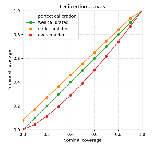
For a nominal coverage level \(c\), CaliBrain evaluates whether the true source value falls inside the corresponding posterior interval or ellipsoid. Empirical coverage is then estimated over many sources or many runs:

\[\hat{g}(c) = \frac{1}{N} \sum_{i=1}^{N} \mathbf{1}\left[x_i^{\mathrm{true}} \in C_i(c)\right].\]

Perfect calibration means \(\hat{g}(c) \approx c\) across the nominal coverage grid. If the empirical curve falls below the diagonal, the posterior uncertainty is too narrow on average; if it falls above the diagonal, it is too wide on average.

nominal = np.linspace(0.0, 1.0, 11)
well_calibrated = nominal
underconfident = np.clip(0.08 + 0.95 * nominal, 0.0, 1.0)
overconfident = nominal**1.35

fig, ax = plt.subplots(figsize=(5.2, 5.0))
ax.plot([0, 1], [0, 1], "--", color="0.4", lw=1.5, label="perfect calibration")
ax.plot(nominal, well_calibrated, "o-", color="#2ca02c", label="well calibrated")
ax.plot(nominal, underconfident, "o-", color="#ff7f0e", label="underconfident")
ax.plot(nominal, overconfident, "o-", color="#d62728", label="overconfident")
ax.set(
    xlabel="Nominal coverage",
    ylabel="Empirical coverage",
    xlim=(0, 1),
    ylim=(0, 1),
    title="Calibration curves",
)
ax.set_aspect("equal", adjustable="box")
ax.grid(True, linestyle="--", alpha=0.4)
ax.legend(loc="upper left")
fig.tight_layout()

Uncertainty representations used in CaliBrain

CaliBrain does not calibrate every solver output in the same geometric form. The uncertainty object depends on the source model and on how the posterior covariance is reduced before calibration:

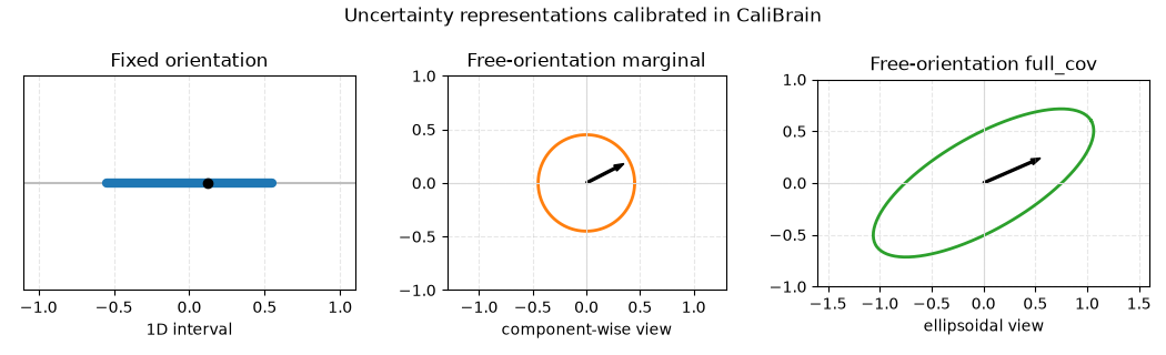
• Fixed orientation uses one scalar posterior variance per source. The calibrated object is therefore a one-dimensional credible interval around the posterior mean. If \(\hat{x}_i\) is the posterior mean and \(\sigma_i^2\) is the posterior variance, then the interval at nominal coverage \(c\) is constructed from the corresponding Gaussian quantile. Coverage asks whether the true scalar source value lies inside that interval.

• Free-orientation ``marginal`` mode treats each orientation component separately. For EEG this means three component-wise intervals per source; for reduced free-orientation MEG it means two. This representation uses only marginal variances and ignores covariance between orientation components. It is therefore simpler and cheaper to evaluate, but it does not represent the full local posterior geometry.

• Free-orientation ``full_cov`` mode uses a local covariance block for each source and constructs a multivariate credible set. Geometrically, this is an ellipsoid centered at the local posterior mean. Coverage asks whether the true orientation vector lies inside that ellipsoid. This representation preserves correlation structure between orientation components and is the more faithful local posterior description.

In the current workflow, calibration is typically performed on temporally aggregated summaries. Posterior means are averaged over time, and posterior covariance is correspondingly reduced to a source-level uncertainty object. The calibration problem is therefore formulated on source summaries rather than on the full source-by-time posterior.

These representations are constructed by uncertainty estimation.

angle = np.linspace(0, 2 * np.pi, 200)
circle_x = 0.45 * np.cos(angle)
circle_y = 0.45 * np.sin(angle)
ellipse_x = 1.2 * np.cos(angle)
ellipse_y = 0.45 * np.sin(angle)
rotation = np.deg2rad(30)
ellipse_rot_x = ellipse_x * np.cos(rotation) - ellipse_y * np.sin(rotation)
ellipse_rot_y = ellipse_x * np.sin(rotation) + ellipse_y * np.cos(rotation)

fig, axes = plt.subplots(1, 3, figsize=(10.5, 3.2))

axes[0].plot([-1.1, 1.1], [0, 0], color="0.75")
axes[0].plot([-0.55, 0.55], [0, 0], lw=6, color="#1f77b4", solid_capstyle="round")
axes[0].plot(0.12, 0, "o", color="k")
axes[0].set_title("Fixed orientation")
axes[0].set_xlim(-1.1, 1.1)
axes[0].set_ylim(-0.5, 0.5)
axes[0].set_yticks([])
axes[0].set_xlabel("1D interval")

axes[1].plot(circle_x, circle_y, color="#ff7f0e", lw=2)
axes[1].arrow(0, 0, 0.35, 0.18, width=0.02, color="k", length_includes_head=True)
axes[1].set_title("Free-orientation marginal")
axes[1].set_aspect("equal", adjustable="box")
axes[1].set_xlim(-1.3, 1.3)
axes[1].set_ylim(-1.0, 1.0)
axes[1].set_xlabel("component-wise view")

axes[2].plot(ellipse_rot_x, ellipse_rot_y, color="#2ca02c", lw=2)
axes[2].arrow(0, 0, 0.55, 0.24, width=0.02, color="k", length_includes_head=True)
axes[2].set_title("Free-orientation full_cov")
axes[2].set_aspect("equal", adjustable="box")
axes[2].set_xlim(-1.6, 1.6)
axes[2].set_ylim(-1.0, 1.0)
axes[2].set_xlabel("ellipsoidal view")

for ax in axes[1:]:
    ax.axhline(0, color="0.85", lw=0.8)
    ax.axvline(0, color="0.85", lw=0.8)

for ax in axes:
    ax.grid(True, linestyle="--", alpha=0.3)

fig.suptitle("Uncertainty representations calibrated in CaliBrain")
fig.tight_layout()

Recalibration by isotonic regression

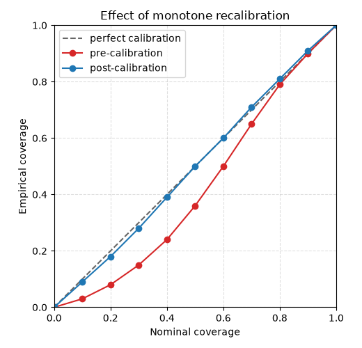
When the raw empirical coverage curve is systematically misaligned with the diagonal, CaliBrain applies a monotone recalibration map learned by isotonic regression. The goal is not to change the posterior mean, but to correct the nominal-to-empirical coverage relationship.

In the current documentation and workflows, post-calibration is illustrated through the workflow modes post_oracle, post_pooled, post_pooled_mismatch, and post_fixed. These are not different regression models. They are different examples of how train and evaluation splits are chosen around the same isotonic recalibration step.

More concretely, CaliBrain first computes a pre-calibration empirical curve \(\hat{g}(c)\) on a training split. Isotonic regression then fits a monotone map between nominal and empirical coverage levels. The monotonicity constraint is essential: coverage should not decrease when the nominal set size increases. The fitted map is then used to obtain recalibrated nominal levels on the evaluation split. In this way, post-calibration changes the interpretation of the nominal coverage grid rather than changing the inverse solution itself.

This is useful because raw posterior uncertainty is often systematically miscalibrated but still ordered sensibly. For example, wider posterior sets may indeed correspond to higher empirical coverage, yet not at the correct nominal levels. Isotonic regression preserves that ordering while correcting the nominal-to-empirical mismatch.

Evaluation is broader than these named workflow modes. One may evaluate raw empirical coverage, recalibrated coverage, summary calibration metrics, source-reconstruction error, uncertainty magnitude, or transfer across conditions. The named modes organize common benchmark scenarios; they do not exhaust the possible analyses.

pre_curve = np.array([0.0, 0.03, 0.08, 0.15, 0.24, 0.36, 0.5, 0.65, 0.79, 0.9, 1.0])
post_curve = np.array([0.0, 0.09, 0.18, 0.28, 0.39, 0.5, 0.6, 0.71, 0.81, 0.91, 1.0])

fig, ax = plt.subplots(figsize=(5.2, 5.0))
ax.plot([0, 1], [0, 1], "--", color="0.4", lw=1.5, label="perfect calibration")
ax.plot(nominal, pre_curve, "o-", color="#d62728", label="pre-calibration")
ax.plot(nominal, post_curve, "o-", color="#1f77b4", label="post-calibration")
ax.set(
    xlabel="Nominal coverage",
    ylabel="Empirical coverage",
    xlim=(0, 1),
    ylim=(0, 1),
    title="Effect of monotone recalibration",
)
ax.set_aspect("equal", adjustable="box")
ax.grid(True, linestyle="--", alpha=0.4)
ax.legend(loc="upper left")
fig.tight_layout()

Distinguishing settings in CaliBrain

CaliBrain distinguishes uncertainty and calibration problems along two main axes.

1. Fixed versus free orientation

In fixed orientation, each source location is represented by a single scalar coefficient. Uncertainty is therefore one-dimensional at each source, and calibration is based on scalar posterior variances and scalar coverage intervals.

In free orientation, each source location is represented by a vector of orientation components. For EEG this is typically three-dimensional; for the reduced free-orientation MEG setting used here it is two-dimensional. The local uncertainty object is therefore multivariate. CaliBrain can either calibrate this using component-wise marginal intervals or using local full_cov ellipsoids.

2. EEG versus MEG

EEG and MEG differ through the forward model and the orientation convention used in the package. In the current documentation:

• free-orientation EEG uses 3-component source vectors and therefore admits both marginal and full_cov local uncertainty representations;

• reduced free-orientation MEG uses 2-component tangential vectors, changing both the geometry of the local uncertainty set and the dimensionality of the coverage test;

• fixed-orientation analyses for EEG and MEG share the same scalar coverage logic, but the leadfield and sensor units differ.

As a consequence, calibration curves should only be compared across settings with care. A fixed-orientation scalar interval, a free-orientation component-wise interval, and a free-orientation ellipsoid are not the same uncertainty object. They answer related but distinct coverage questions.

This is why CaliBrain keeps orientation type, modality, uncertainty representation, and calibration mode explicit throughout the workflow.