03. Leadfield Construction

This tutorial mainly explains the LeadfieldBuilder class. It demonstrates the three leadfield retrieval modes used by LeadfieldBuilder:

• retrieve_mode="random": create a synthetic random leadfield;

• retrieve_mode="simulate": run a simulation pipeline;

• retrieve_mode="load": load a leadfield through the standard loading API.

The full MNE simulation pipeline requires subject surfaces, BEM files, sensor information, and forward-solution configuration. To keep this tutorial executable during documentation builds, the simulate example uses a small subclass that returns a deterministic synthetic leadfield while preserving the same get_leadfield(..., retrieve_mode="simulate") interface.

Scientific motivation

A leadfield maps source amplitudes to sensor measurements. In fixed orientation, the leadfield has shape (n_sensors, n_sources). In free orientation, CaliBrain represents it as (n_sensors, n_sources, n_components).

Units matter because the leadfield connects source dipole moments to sensor measurements:

• source amplitudes are represented in nAm;

• MEG magnetometer leadfields are typically reported in fT / nAm;

• EEG leadfields are typically reported in µV / nAm.

import matplotlib.pyplot as plt
import numpy as np
from mne.io.constants import FIFF
from tempfile import TemporaryDirectory

from calibrain import LeadfieldBuilder
from calibrain.utils import get_data_path


RANDOM_SEED = 23

Use the CaliBrain data-root helper

CaliBrain resolves local datasets with get_data_path. With no argument, it uses CALIBRAIN_DATA if the environment variable is set, otherwise the repository-level data directory.

data_root = get_data_path()
leadfield_dir = data_root / "1284src_leadfield"

print("tutorial data root:", data_root)
print("tutorial leadfield directory:", leadfield_dir)

tutorial data root: /home/docs/checkouts/readthedocs.org/user_builds/calibrain/checkouts/dev/data
tutorial leadfield directory: /home/docs/checkouts/readthedocs.org/user_builds/calibrain/checkouts/dev/data/1284src_leadfield

Random retrieval mode

retrieve_mode="random" is useful for lightweight tests. It does not represent a physical head model. The generated values are arbitrary unless explicit metadata and scaling are attached later.

builder = LeadfieldBuilder(leadfield_dir=leadfield_dir)

random_fixed = builder.get_leadfield(
    subject="demo",
    orientation_type="fixed",
    retrieve_mode="random",
    n_sensors=12,
    n_sources=24,
    return_metadata=True,
)

random_free = builder.get_leadfield(
    subject="demo",
    orientation_type="free",
    retrieve_mode="random",
    n_sensors=12,
    n_sources=24,
    return_metadata=True,
)

print("random fixed shape:", random_fixed.leadfield.shape)
print("random free shape:", random_free.leadfield.shape)

random fixed shape: (12, 24)
random free shape: (12, 24, 3)

Simulate retrieval mode

In production, retrieve_mode="simulate" runs the full MNE-based pipeline: source space, BEM model, sensor info, forward solution, and leadfield extraction. That path requires external anatomy and MNE configuration, so this lightweight tutorial shows the expected output structure with a synthetic stand-in that matches the usual fixed-orientation shape and metadata.

rng = np.random.default_rng(RANDOM_SEED)
n_sensors = 12
n_sources = 24
source_positions = rng.normal(scale=0.04, size=(n_sources, 3))
sensor_positions = rng.normal(scale=0.08, size=(n_sensors, 3))
distances = np.linalg.norm(
    sensor_positions[:, None, :] - source_positions[None, :, :],
    axis=2,
)
simulated_leadfield = 1.0 / np.maximum(distances, 0.02) ** 2
simulated_leadfield *= rng.choice([-1.0, 1.0], size=simulated_leadfield.shape)
simulated_leadfield /= np.linalg.norm(simulated_leadfield, axis=0, keepdims=True)
simulated_q_basis = np.eye(n_sources)

print("simulate-like shape:", simulated_leadfield.shape)
print("simulate-like sensor unit:", FIFF.FIFF_UNIT_T)
print("simulate-like sensor unit multiplier:", FIFF.FIFF_UNITM_F)
print("simulate-like coil type:", FIFF.FIFFV_COIL_VV_MAG_T1)

simulate-like shape: (12, 24)
simulate-like sensor unit: 112 (FIFF_UNIT_T)
simulate-like sensor unit multiplier: -15 (FIFF_UNITM_F)
simulate-like coil type: 3022 (FIFFV_COIL_VV_MAG_T1)

Exercise the load interface

In the full workflow, retrieve_mode="load" reads a precomputed leadfield dataset from leadfield_dir. Here we create a temporary fixture and then load it through the standard LeadfieldBuilder API.

tmpdir = TemporaryDirectory()
temp_builder = LeadfieldBuilder(leadfield_dir=tmpdir.name)
np.savez(
    f"{tmpdir.name}/demo_subject_fixed_leadfield.npz",
    leadfield=simulated_leadfield,
    sensor_kind=FIFF.FIFFV_MEG_CH,
    sensor_units=FIFF.FIFF_UNIT_T,
    sensor_unitmult=FIFF.FIFF_UNITM_F,
    coil_type=FIFF.FIFFV_COIL_VV_MAG_T1,
    src_coords=source_positions,
    Q_basis=simulated_q_basis,
)
loaded = temp_builder.get_leadfield(
    subject="demo_subject",
    orientation_type="fixed",
    retrieve_mode="load",
    return_metadata=True,
)

print("loaded shape:", loaded.leadfield.shape)
print("loaded equals simulate-like:", np.allclose(loaded.leadfield, simulated_leadfield))

loaded shape: (12, 24)
loaded equals simulate-like: True

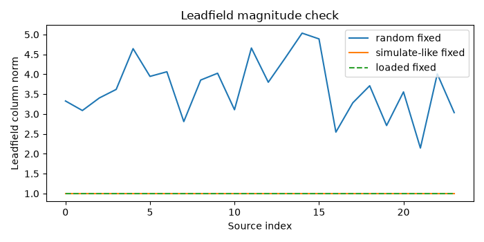
Visualize leadfield magnitudes

A simple quality-control plot is the per-source leadfield norm. Large deviations can indicate scaling, orientation, or file-loading problems.

fig, ax = plt.subplots(figsize=(7, 3.5))
ax.plot(np.linalg.norm(random_fixed.leadfield, axis=0), label="random fixed")
ax.plot(np.linalg.norm(simulated_leadfield, axis=0), label="simulate-like fixed")
ax.plot(np.linalg.norm(loaded.leadfield, axis=0), "--", label="loaded fixed")
ax.set(
    xlabel="Source index",
    ylabel="Leadfield column norm",
    title="Leadfield magnitude check",
)
ax.legend(loc="best")
fig.tight_layout()

Summary

The retrieval modes serve different purposes:

• random: fast synthetic matrices for testing shape logic;

• simulate: full MNE forward-model construction in production;

• load: standard workflow mode for precomputed leadfield datasets.

For paper-scale workflows, use get_data_path to locate the local dataset root and point LeadfieldBuilder to the directory containing *_fixed_leadfield.npz or *_free_leadfield.npz files.