02. Source Simulation

This tutorial mainly explains the SourceSimulator class. It demonstrates CaliBrain source-level simulation under several configurations. It creates sparse ERP-like source time courses for fixed orientation, free-orientation EEG, and free-orientation MEG, then visualizes the active sources.

Source simulation is the first numerical step in the CaliBrain workflow. Later tutorials project these source signals through a leadfield to create sensor-level data.

Scientific motivation

In simulation-based calibration experiments, the true source activity is known. This allows CaliBrain to compare inverse estimates and uncertainty intervals against ground truth. The source simulator creates sparse event-related potential (ERP)-like signals: only nnz source locations are active, while the remaining locations are exactly zero.

Units

CaliBrain source amplitudes are dipole moments. Internally, SourceSimulator labels the output as ampere meter with nano scaling:

• simulator.units == FIFF.FIFF_UNIT_AM;

• simulator.unitmult == FIFF.FIFF_UNITM_N.

Numerically, the simulated values are expressed in nAm. The amplitude_distribution therefore controls peak dipole moments in nAm.

import matplotlib.pyplot as plt
import numpy as np
from mne.io.constants import FIFF

from calibrain import SourceSimulator


RANDOM_SEED = 13

Configure ERP-like source waveforms

SourceSimulator uses an ERP configuration to define the time axis, stimulus onset, bandpass range, amplitude distribution, and timing behavior. The key parameters are:

• tmin / tmax: epoch start and end in seconds;

• stim_onset: stimulus time in seconds;

• sfreq: sampling frequency in Hz;

• fmin / fmax: bandpass range used to shape the ERP waveform;

• amplitude_distribution: log-normal peak amplitude distribution in nAm;

• random_erp_timing: whether ERP duration/onset varies across sources;

• erp_min_length: minimum ERP segment length in samples.

base_erp_config = {
    "tmin": -0.1,
    "tmax": 0.8,
    "stim_onset": 0.0,
    "sfreq": 100,
    "fmin": 2,
    "fmax": 8,
    "amplitude_distribution": {
        "median": 10.0,
        "sigma": 0.15,
        "clip": [2.0, 25.0],
    },
    "random_erp_timing": False,
    "erp_min_length": 20,
}

simulator = SourceSimulator(ERP_config=base_erp_config)
times = np.arange(
    base_erp_config["tmin"],
    base_erp_config["tmax"],
    1.0 / base_erp_config["sfreq"],
)

print("source unit:", simulator.units)
print("source unit multiplier:", simulator.unitmult)

source unit: 202 (FIFF_UNIT_AM)
source unit multiplier: -9 (FIFF_UNITM_N)

Define source-space configurations

n_sources is the number of candidate source locations. nnz is the number of non-zero locations. orientation_type controls the output shape:

• fixed orientation: one scalar coefficient per source;

• free EEG orientation: three local components per source;

• free MEG orientation: two local components per source.

The MEG free-orientation reduction reflects that magnetometer/gradiometer leadfields are represented in the two-dimensional MEG-sensitive subspace.

source_configs = {
    "fixed": {
        "n_sources": 40,
        "nnz": 4,
        "orientation_type": "fixed",
        "coil_type": None,
        "seed": RANDOM_SEED,
    },
    "free_eeg": {
        "n_sources": 40,
        "nnz": 4,
        "orientation_type": "free",
        "coil_type": FIFF.FIFFV_COIL_EEG,
        "seed": RANDOM_SEED,
    },
    "free_meg": {
        "n_sources": 40,
        "nnz": 4,
        "orientation_type": "free",
        "coil_type": FIFF.FIFFV_COIL_VV_MAG_T1,
        "seed": RANDOM_SEED,
    },
}
x_fixed, active_fixed = simulator.simulate(
    n_sources=source_configs["fixed"]["n_sources"],
    nnz=source_configs["fixed"]["nnz"],
    orientation_type=source_configs["fixed"]["orientation_type"],
    seed=source_configs["fixed"]["seed"],
)
print(f"{'fixed':>11} shape: {x_fixed.shape}; active sources: {active_fixed}")

x_free_eeg, active_free_eeg = simulator.simulate(
    n_sources=source_configs["free_eeg"]["n_sources"],
    nnz=source_configs["free_eeg"]["nnz"],
    orientation_type=source_configs["free_eeg"]["orientation_type"],
    coil_type=source_configs["free_eeg"]["coil_type"],
    seed=source_configs["free_eeg"]["seed"],
)
print(f"{'free_eeg':>11} shape: {x_free_eeg.shape}; active sources: {active_free_eeg}")

x_free_meg, active_free_meg = simulator.simulate(
    n_sources=source_configs["free_meg"]["n_sources"],
    nnz=source_configs["free_meg"]["nnz"],
    orientation_type=source_configs["free_meg"]["orientation_type"],
    coil_type=source_configs["free_meg"]["coil_type"],
    seed=source_configs["free_meg"]["seed"],
)
print(f"{'free_meg':>11} shape: {x_free_meg.shape}; active sources: {active_free_meg}")

   fixed shape: (40, 90); active sources: [30 17 23 32]
free_eeg shape: (40, 3, 90); active sources: [30 17 23 32]
free_meg shape: (40, 2, 90); active sources: [30 17 23 32]

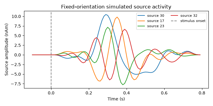
Fixed-orientation example

Fixed orientation represents each source location with one scalar time course. The returned source matrix has shape (n_sources, n_times).

fig, ax = plt.subplots(figsize=(7, 3.5))
for src_idx in active_fixed:
    ax.plot(times, x_fixed[src_idx], label=f"source {src_idx}")
ax.axvline(
    base_erp_config["stim_onset"],
    color="0.5",
    linestyle="--",
    label="stimulus onset",
)
ax.set(
    xlabel="Time (s)",
    ylabel="Source amplitude (nAm)",
    title="Fixed-orientation simulated source activity",
)
ax.legend(loc="upper right", ncols=2, fontsize=8)
fig.tight_layout()

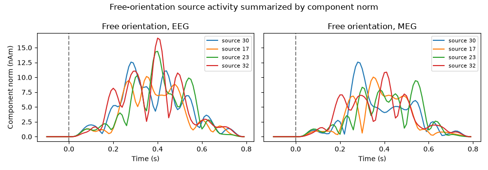
EEG and MEG free-orientation examples

Free orientation represents each source location with multiple local components. For EEG, CaliBrain uses three components. For MEG magnetometers or gradiometers, it uses two components in the MEG-sensitive subspace.

For free orientation, plotting every component can be visually crowded. A compact summary is the Euclidean norm across orientation components for each active source.

free_eeg_norm = np.linalg.norm(x_free_eeg, axis=1)
free_meg_norm = np.linalg.norm(x_free_meg, axis=1)

fig, axes = plt.subplots(1, 2, figsize=(10, 3.5), sharex=True, sharey=True)
for src_idx in active_free_eeg:
    axes[0].plot(times, free_eeg_norm[src_idx], label=f"source {src_idx}")
axes[0].set_title("Free orientation, EEG")
axes[0].set_xlabel("Time (s)")
axes[0].set_ylabel("Component norm (nAm)")
axes[0].axvline(base_erp_config["stim_onset"], color="0.5", linestyle="--")

for src_idx in active_free_meg:
    axes[1].plot(times, free_meg_norm[src_idx], label=f"source {src_idx}")
axes[1].set_title("Free orientation, MEG")
axes[1].set_xlabel("Time (s)")
axes[1].axvline(base_erp_config["stim_onset"], color="0.5", linestyle="--")

for ax in axes:
    ax.legend(loc="upper right", fontsize=8)

fig.suptitle("Free-orientation source activity summarized by component norm")
fig.tight_layout()

What this stage produces

Source simulation returns arrays and active-source indices:

• fixed orientation: x with shape (n_sources, n_times), in nAm;

• free EEG orientation: x with shape (n_sources, 3, n_times), in nAm per local component;

• free MEG orientation: x with shape (n_sources, 2, n_times), in nAm per retained MEG-sensitive component.

The next step is leadfield generation/loading, followed by sensor simulation.