01. Introduction

CaliBrain studies whether posterior uncertainty estimates in M/EEG inverse source imaging are empirically calibrated. In a calibrated model, intervals requested at nominal coverage c should contain the true simulated source activity approximately c of the time.

This first tutorial serves as both the introduction and the scientific background entry point for the runnable gallery. It uses lightweight synthetic fixed-orientation source arrays so that the gallery build remains fast and reproducible.

Scientific question

M/EEG inverse problems are ill posed: multiple source configurations can explain the same sensor data. A useful inverse method should therefore report uncertainty, not only a point estimate. CaliBrain evaluates that uncertainty through coverage calibration.

Here we construct the minimal objects required for a calibration curve:

• x_true: simulated ground-truth source activity,

• x_hat: posterior mean estimate,

• posterior_var: source-wise posterior variance.

import matplotlib.pyplot as plt
import numpy as np

from calibrain import UncertaintyEstimator


RANDOM_SEED = 7

rng = np.random.default_rng(RANDOM_SEED)

Simulate sparse fixed-orientation source activity

The source matrix has shape (n_sources, n_times). Most sources are zero; a small subset contains ERP-like activity. Later tutorials replace this toy construction with SourceSimulator and full workflow outputs.

n_sources = 48
n_times = 80
time = np.linspace(-0.2, 0.5, n_times)

x_true = np.zeros((n_sources, n_times))
active_sources = rng.choice(n_sources, size=5, replace=False)
erp_waveform = np.exp(-0.5 * ((time - 0.12) / 0.045) ** 2)
x_true[active_sources] = rng.normal(1.0, 0.2, size=(5, 1)) * erp_waveform

Create a simple posterior estimate

In real workflows, inverse solvers such as gamma_map_sflex or BMN produce posterior means and covariance estimates. This first tutorial uses controlled synthetic posterior statistics so the calibration concept is isolated from solver details.

posterior_var = np.full(n_sources, 0.06**2)
x_hat = x_true + rng.normal(
    loc=0.0,
    scale=np.sqrt(posterior_var)[:, None],
    size=x_true.shape,
)

Compute empirical coverage

UncertaintyEstimator constructs intervals over a nominal coverage grid and reports the empirical fraction of source values covered by those intervals. The aggregated method averages over time before evaluating source-level intervals.

nominal_coverages = np.linspace(0.0, 1.0, 11)
uncertainty = UncertaintyEstimator(nominal_coverages=nominal_coverages)
curve = uncertainty.calibration_curve_intervals_aggregated(
    x_true=x_true,
    x_hat=x_hat,
    posterior_var=posterior_var,
)

print(np.round(curve["empirical_coverages"], 3))

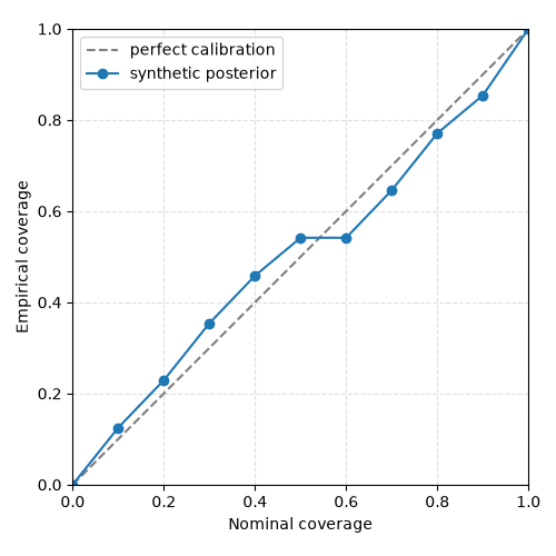
[0.    0.125 0.229 0.354 0.458 0.542 0.542 0.646 0.771 0.854 1.   ]

Plot the calibration curve

The dashed diagonal is perfect calibration. Points below the diagonal indicate undercoverage, i.e. overconfident uncertainty. Points above the diagonal indicate overcoverage, i.e. underconfident uncertainty.

fig, ax = plt.subplots(figsize=(5, 5))
ax.plot([0, 1], [0, 1], "--", color="0.5", label="perfect calibration")
ax.plot(
    curve["nominal_coverages"],
    curve["empirical_coverages"],
    "o-",
    label="synthetic posterior",
)
ax.set(
    xlabel="Nominal coverage",
    ylabel="Empirical coverage",
    xlim=(0, 1),
    ylim=(0, 1),
)
ax.set_aspect("equal", adjustable="box")
ax.grid(True, linestyle="--", alpha=0.4)
ax.legend()
fig.tight_layout()

Summary

Production workflows use the same scientific objects but persist them as H5 posterior summaries, manifest CSV files, aggregated NPZ datasets, calibration JSON summaries, and publication figures.