10. Data Generation

This tutorial mainly explains the high-level DataGenerator class.

It shows how DataGenerator orchestrates the upstream pipeline:

• source simulation;

• leadfield loading;

• sensor simulation;

• source estimation;

• tabular run metadata returned as a DataFrame.

Scientific motivation

DataGenerator is the workflow orchestrator behind CaliBrain’s data generation stage. Unlike the lower-level classes, it does not represent one scientific operation. Instead, it runs complete configured experiments over solver, data, and noise settings and returns run-wise metadata that can be passed to downstream workflow stages.

This tutorial uses a tiny synthetic setup so the class can be exercised directly in the documentation build.

from tempfile import TemporaryDirectory

import matplotlib.pyplot as plt
import numpy as np
from mne.io.constants import FIFF

from calibrain import DataGenerator, LeadfieldBuilder, SensorSimulator, SourceSimulator, gamma_map_sflex


RANDOM_SEED = 83
tmpdir = TemporaryDirectory()
FIG_DIR = tmpdir.name

Build a tiny leadfield fixture

DataGenerator expects LeadfieldBuilder to provide leadfields. In the current implementation, its internal data preparation step calls retrieve_mode="load". For a runnable tutorial we therefore provide a deterministic payload through the same high-level builder API.

Units:

• source amplitudes are in nAm;

• source coordinates are represented in m;

• the synthetic EEG leadfield is interpreted as µV / nAm.

rng = np.random.default_rng(RANDOM_SEED)
subject = "demo_subject"
n_sensors = 16
n_sources = 32
src_coords = rng.normal(scale=0.04, size=(n_sources, 3))
leadfield = rng.normal(scale=0.03, size=(n_sensors, n_sources))
leadfield /= np.maximum(
    np.linalg.norm(leadfield, axis=0, keepdims=True),
    np.finfo(float).eps,
)
leadfield *= 0.6
q_basis = np.zeros((n_sources, 3, 0), dtype=float)
print("leadfield shape:", leadfield.shape)
leadfield_dir = TemporaryDirectory()
np.savez(
    f"{leadfield_dir.name}/{subject}_fixed_leadfield.npz",
    leadfield=leadfield,
    sensor_kind=FIFF.FIFFV_EEG_CH,
    sensor_units=FIFF.FIFF_UNIT_V,
    sensor_unitmult=FIFF.FIFF_UNITM_MU,
    coil_type=FIFF.FIFFV_COIL_EEG,
    src_coords=src_coords,
    Q_basis=q_basis,
)

leadfield shape: (16, 32)

Configure the generator

The class is configured from three grids:

• solver_param_grid for estimator hyperparameters;

• data_param_grid for source/sensor-generation settings;

• noise_param_grid for workflow noise handling.

Here we keep them deliberately small. Two alpha_SNR values produce two runs with otherwise matched settings.

erp_config = {
    "tmin": -0.1,
    "tmax": 0.8,
    "stim_onset": 0.0,
    "sfreq": 100,
    "fmin": 2,
    "fmax": 8,
    "amplitude_distribution": {
        "median": 8.0,
        "sigma": 0.15,
        "clip": [2.0, 20.0],
    },
    "random_erp_timing": False,
    "erp_min_length": 20,
}

source_simulator = SourceSimulator(ERP_config=erp_config)
leadfield_builder = LeadfieldBuilder(leadfield_dir=leadfield_dir.name)
sensor_simulator = SensorSimulator()

generator = DataGenerator(
    solver=gamma_map_sflex,
    solver_param_grid={
        "sigma": [0.01],
        "max_iter": [150],
        "tol": [1e-7],
    },
    data_param_grid={
        "subject": [subject],
        "nnz": [4],
        "orientation_type": ["fixed"],
        "alpha_SNR": [0.5, 0.8],
        "sensor_white_noise_std": [0.2],
    },
    noise_param_grid={
        "noise_type": ["oracle"],
    },
    ERP_config=erp_config,
    source_simulator=source_simulator,
    leadfield_builder=leadfield_builder,
    sensor_simulator=sensor_simulator,
    save_posterior_stats=False,
    random_state=RANDOM_SEED,
)

Run the generator

DataGenerator.run returns a pandas.DataFrame with one row per run. Each row includes solver metadata, source/sensor settings, and run-level diagnostics.

results = generator.run(
    nruns=1,
    fig_path=FIG_DIR,
    n_jobs=1,
)

print("result columns:", list(results.columns))
print(results[["global_run_id", "solver", "noise_type", "alpha_SNR", "nnz"]])

2026-06-15 09:38:11 - INFO - [run: 1/1 | config: 1/2 | total: 1/2] gamma_map_sflex | oracle | 4 NNZ | 0.5 SNR
2026-06-15 09:38:11 - INFO - [run: 1/1 | config: 2/2 | total: 2/2] gamma_map_sflex | oracle | 4 NNZ | 0.8 SNR
result columns: ['run_id', 'global_run_id', 'seed', 'solver', 'noise_type', 'max_iter', 'sigma', 'tol', 'alpha_SNR', 'nnz', 'orientation_type', 'sensor_white_noise_std', 'subject', 'sensor_kind', 'coil_type', 'n_sources', 'n_times', 'gamma', 'noise_var', 'active_indices_size']
   global_run_id           solver noise_type  alpha_SNR  nnz
0              1  gamma_map_sflex     oracle        0.5    4
1              2  gamma_map_sflex     oracle        0.8    4

What DataGenerator produces directly

At class level, the direct products are:

• one row per run in the returned DataFrame;

• solver, source, and sensor metadata needed to compare runs.

Full workflow scripts can additionally persist summaries for later aggregation and calibration. This tutorial stays at class level and focuses on the direct in-memory products of the class itself.

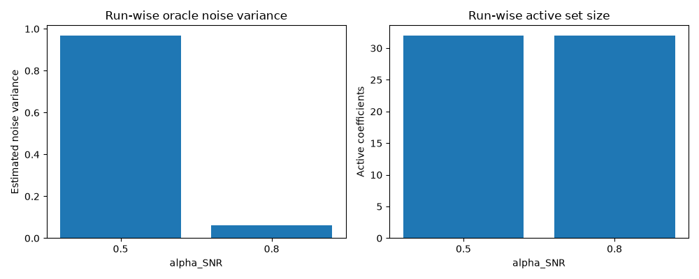
Plot a small run summary

This simple plot summarizes how the two tutorial runs differ in noise level and active-set size.

fig, axes = plt.subplots(1, 2, figsize=(10, 4))
alpha_labels = results["alpha_SNR"].astype(str).tolist()
xpos = np.arange(len(alpha_labels))
axes[0].bar(xpos, results["noise_var"])
axes[0].set(
    xlabel="alpha_SNR",
    ylabel="Estimated noise variance",
    title="Run-wise oracle noise variance",
    xticks=xpos,
    xticklabels=alpha_labels,
)

axes[1].bar(xpos, results["active_indices_size"])
axes[1].set(
    xlabel="alpha_SNR",
    ylabel="Active coefficients",
    title="Run-wise active set size",
    xticks=xpos,
    xticklabels=alpha_labels,
)
fig.tight_layout()

Summary

DataGenerator is the high-level class that orchestrates the upstream workflow. In this tutorial it:

• loaded a leadfield through the standard builder API;

• simulated source and sensor data;

• ran gamma_map_sflex;

• returned run metadata as a table.

This is the class-level precursor to the full workflow, where the same runs are repeated systematically across parameter grids.