05. Source Estimation

This tutorial mainly explains the SourceEstimator class. It demonstrates the current CaliBrain source-estimation interface using the active inverse solvers that are still part of the pipeline:

• gamma_map_sflex for sparse Bayesian estimation with an sFLEX basis;

• gamma_lambda_map_sflex for the sFLEX variant with joint noise learning;

• BMN for Bayesian minimum-norm estimation with fixed noise variance;

• BMN_joint for Bayesian minimum-norm estimation with joint noise learning.

The examples cover:

• fixed-orientation source estimation;

• comparison of sparse and minimum-norm posterior summaries;

• free-orientation EEG source estimation with a 3-component leadfield;

• explicit use of the workflow noise modes oracle, baseline, and adaptive_joint_learning.

Scientific motivation

Source estimation in CaliBrain reconstructs latent source activity x from sensor measurements y and a leadfield L:

y = L x + noise

The output is not only a point estimate. Current solvers return posterior summaries that are later consumed by uncertainty estimation and calibration:

• posterior_mean: reconstructed source time courses;

• posterior_cov: posterior covariance in coefficient space;

• solver-specific diagnostics such as active sets, learned hyperparameters, or learned noise levels.

Units remain consistent across the workflow:

• source amplitudes are simulated in nAm;

• EEG leadfields are interpreted as µV / nAm;

• source coordinates for sFLEX are in m;

• resulting sensor traces are therefore in µV.

import matplotlib.pyplot as plt
import numpy as np
from mne.io.constants import FIFF

from calibrain import (
    BMN,
    BMN_joint,
    SensorSimulator,
    SourceEstimator,
    SourceSimulator,
    gamma_lambda_map_sflex,
    gamma_map_sflex,
)


RANDOM_SEED = 41

Build a lightweight simulation setup

The source simulator generates sparse ERP-like activity. We then construct small synthetic EEG leadfields so the tutorial runs quickly during docs builds.

The parameter meanings are the same as in the source-simulation tutorial:

• tmin and tmax define the simulated time window in seconds;

• stim_onset marks the ERP onset;

• sfreq is the sampling frequency in Hz;

• amplitude_distribution controls source amplitudes in nAm.

For the sFLEX solvers we also need source coordinates. Here they are small synthetic positions in meters. sigma=0.01 therefore means a spatial scale of 10 mm.

erp_config = {
    "tmin": -0.1,
    "tmax": 0.8,
    "stim_onset": 0.0,
    "sfreq": 100,
    "fmin": 2,
    "fmax": 8,
    "amplitude_distribution": {
        "median": 8.0,
        "sigma": 0.15,
        "clip": [2.0, 20.0],
    },
    "random_erp_timing": False,
    "erp_min_length": 20,
}

times = np.arange(erp_config["tmin"], erp_config["tmax"], 1.0 / erp_config["sfreq"])
source_simulator = SourceSimulator(ERP_config=erp_config)
sensor_simulator = SensorSimulator()

rng = np.random.default_rng(RANDOM_SEED)
n_sensors = 16
n_sources = 32
src_coords = rng.normal(scale=0.04, size=(n_sources, 3))

leadfield_fixed = rng.normal(scale=0.03, size=(n_sensors, n_sources))
leadfield_fixed /= np.maximum(
    np.linalg.norm(leadfield_fixed, axis=0, keepdims=True),
    np.finfo(float).eps,
)
leadfield_fixed *= 0.6

leadfield_free_eeg = rng.normal(scale=0.015, size=(n_sensors, n_sources, 3))
leadfield_free_eeg /= np.maximum(
    np.linalg.norm(leadfield_free_eeg, axis=0, keepdims=True),
    np.finfo(float).eps,
)
leadfield_free_eeg *= 0.4

sensor_simulator.set_sensor_metadata(
    kind=FIFF.FIFFV_EEG_CH,
    units=FIFF.FIFF_UNIT_V,
    unitmult=FIFF.FIFF_UNITM_MU,
    coil_type=FIFF.FIFFV_COIL_EEG,
)

Fixed-orientation example

Fixed orientation uses one coefficient per source, so the leadfield has shape (n_sensors, n_sources) and the posterior mean has shape (n_sources, n_times).

x_true_fixed, active_fixed = source_simulator.simulate(
    n_sources=n_sources,
    nnz=4,
    orientation_type="fixed",
    seed=RANDOM_SEED,
)

y_fixed_clean, y_fixed_noisy, fixed_noise, fixed_eta = sensor_simulator.simulate(
    x=x_true_fixed,
    L=leadfield_fixed,
    alpha_SNR=0.7,
    sensor_white_noise_std=0.2,
    seed=RANDOM_SEED,
)

tmin = erp_config["tmin"]
stim_onset = erp_config["stim_onset"]
sfreq = erp_config["sfreq"]
pre_stimulus_onset = int((stim_onset - tmin) * sfreq)
y_fixed_pre = y_fixed_noisy[:, :pre_stimulus_onset]

oracle_noise_var = float(np.var(fixed_noise))
baseline_noise_var = float(np.mean(np.std(y_fixed_pre, axis=1) ** 2))

print("fixed source shape:", x_true_fixed.shape)
print("fixed sensor shape:", y_fixed_noisy.shape)
print("fixed active sources:", active_fixed)
print("fixed eta:", fixed_eta)
print("oracle noise variance:", oracle_noise_var)
print("baseline noise variance:", baseline_noise_var)
print("adaptive joint learning noise variance:", None)

fixed source shape: (32, 90)
fixed sensor shape: (16, 90)
fixed active sources: [11 31 10 24]
fixed eta: 1.82281324753165
oracle noise variance: 0.1397447217185092
baseline noise variance: 0.11194502692152937
adaptive joint learning noise variance: None

Workflow noise modes

The active workflow uses three named noise modes:

• oracle: use var(noise) from the injected sensor noise;

• baseline: estimate variance from the pre-stimulus sensor segment;

• adaptive_joint_learning: pass noise_var=None and let the solver learn a common noise level jointly from the data.

The code below uses these names directly in the solver comparison.

solver_outputs = {}
solver_specs = [
    (
        "gamma_map_sflex_oracle",
        gamma_map_sflex,
        {"max_iter": 150, "tol": 1e-7, "sigma": 0.01, "src_coords": src_coords},
        oracle_noise_var,
    ),
    (
        "gamma_map_sflex_baseline",
        gamma_map_sflex,
        {"max_iter": 150, "tol": 1e-7, "sigma": 0.01, "src_coords": src_coords},
        baseline_noise_var,
    ),
    (
        "gamma_lambda_map_sflex_adaptive_joint_learning",
        gamma_lambda_map_sflex,
        {
            "max_iter": 150,
            "tol": 1e-7,
            "sigma": 0.01,
            "src_coords": src_coords,
            "learn_lambda": True,
        },
        None,
    ),
    (
        "BMN_oracle",
        BMN,
        {"max_iter": 300, "tol": 1e-7, "normalization": False},
        oracle_noise_var,
    ),
    (
        "BMN_baseline",
        BMN,
        {"max_iter": 300, "tol": 1e-7, "normalization": False},
        baseline_noise_var,
    ),
    (
        "BMN_joint_adaptive_joint_learning",
        BMN_joint,
        {"max_iter": 300, "tol": 1e-7, "normalization": False, "learn_noise": True},
        None,
    ),
]

for name, solver, solver_params, noise_var in solver_specs:
    estimator = SourceEstimator(
        solver=solver,
        solver_params=solver_params,
        noise_var=noise_var,
        n_orient=1,
    )
    estimator.fit(leadfield_fixed, y_fixed_noisy)
    solver_outputs[name] = estimator.predict()

for name, result in solver_outputs.items():
    print(f"{name} result keys:", sorted(result.keys()))
    print(f"{name} posterior_mean shape:", result["posterior_mean"].shape)
    print(f"{name} posterior_cov shape:", result["posterior_cov"].shape)
    print(f"{name} learned or used noise_var:", result.get("noise_var"))

gamma_map_sflex_oracle result keys: ['B_spatial', 'active_indices', 'active_source_indices', 'coefficient_indices', 'gamma', 'gammas_full', 'n_iter', 'n_orient', 'noise_var', 'posterior_cov', 'posterior_cov_coeff', 'posterior_mean', 'posterior_mean_coeff', 'source_indices']
gamma_map_sflex_oracle posterior_mean shape: (32, 90)
gamma_map_sflex_oracle posterior_cov shape: (32, 32)
gamma_map_sflex_oracle learned or used noise_var: 0.1397447217185092
gamma_map_sflex_baseline result keys: ['B_spatial', 'active_indices', 'active_source_indices', 'coefficient_indices', 'gamma', 'gammas_full', 'n_iter', 'n_orient', 'noise_var', 'posterior_cov', 'posterior_cov_coeff', 'posterior_mean', 'posterior_mean_coeff', 'source_indices']
gamma_map_sflex_baseline posterior_mean shape: (32, 90)
gamma_map_sflex_baseline posterior_cov shape: (32, 32)
gamma_map_sflex_baseline learned or used noise_var: 0.11194502692152937
gamma_lambda_map_sflex_adaptive_joint_learning result keys: ['B_operator', 'active_indices', 'coefficient_indices', 'err_gamma_hist', 'gamma', 'gammas_full', 'lambda_mean', 'lambda_mean_hist', 'lambdas', 'n_active_hist', 'noise_var', 'posterior_cov', 'posterior_cov_active', 'posterior_cov_active_coeff', 'posterior_cov_coeff', 'posterior_mean', 'posterior_mean_coeff', 'source_indices']
gamma_lambda_map_sflex_adaptive_joint_learning posterior_mean shape: (32, 90)
gamma_lambda_map_sflex_adaptive_joint_learning posterior_cov shape: (32, 32)
gamma_lambda_map_sflex_adaptive_joint_learning learned or used noise_var: 0.11186522283608982
BMN_oracle result keys: ['active_indices', 'coefficient_indices', 'gamma', 'noise_var', 'posterior_cov', 'posterior_mean', 'source_indices']
BMN_oracle posterior_mean shape: (32, 90)
BMN_oracle posterior_cov shape: (32, 32)
BMN_oracle learned or used noise_var: 0.1397447217185092
BMN_baseline result keys: ['active_indices', 'coefficient_indices', 'gamma', 'noise_var', 'posterior_cov', 'posterior_mean', 'source_indices']
BMN_baseline posterior_mean shape: (32, 90)
BMN_baseline posterior_cov shape: (32, 32)
BMN_baseline learned or used noise_var: 0.11194502692152937
BMN_joint_adaptive_joint_learning result keys: ['active_indices', 'coefficient_indices', 'err_gamma_hist', 'gamma', 'gamma_hist', 'lambda', 'lambda_hist', 'noise_var', 'noise_var_hist', 'posterior_cov', 'posterior_mean', 'source_indices']
BMN_joint_adaptive_joint_learning posterior_mean shape: (32, 90)
BMN_joint_adaptive_joint_learning posterior_cov shape: (32, 32)
BMN_joint_adaptive_joint_learning learned or used noise_var: 2.904477730519163e-13

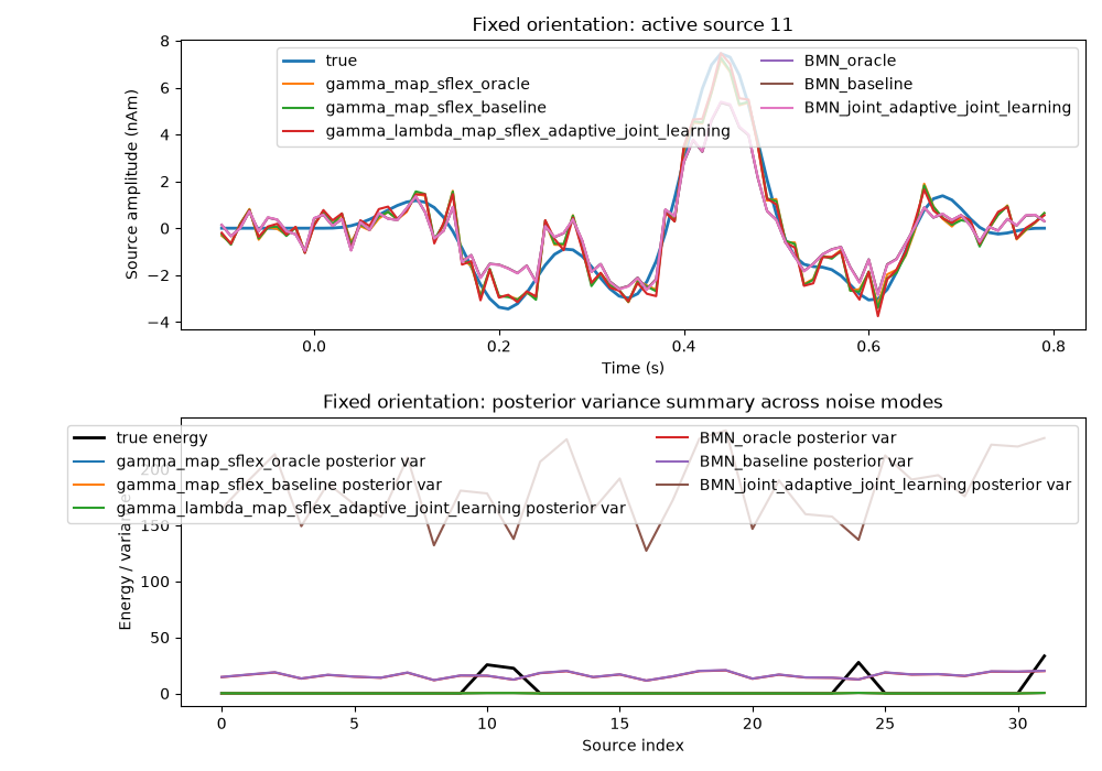
Inspect fixed-orientation posterior summaries

A useful first check is whether the reconstructed activity on a true active source follows the simulated ERP, and how the source-wise posterior variance differs across sparse and minimum-norm estimators under different noise modes.

fixed_source_idx = int(np.atleast_1d(active_fixed)[0])
source_energy_true = np.linalg.norm(x_true_fixed, axis=1)
source_axis = np.arange(n_sources)
plot_order = [
    "gamma_map_sflex_oracle",
    "gamma_map_sflex_baseline",
    "gamma_lambda_map_sflex_adaptive_joint_learning",
    "BMN_oracle",
    "BMN_baseline",
    "BMN_joint_adaptive_joint_learning",
]

fig, axes = plt.subplots(2, 1, figsize=(10, 7), sharex=False)
axes[0].plot(times, x_true_fixed[fixed_source_idx], label="true", linewidth=2)
for name in plot_order:
    axes[0].plot(times, solver_outputs[name]["posterior_mean"][fixed_source_idx], label=name)
axes[0].set(
    xlabel="Time (s)",
    ylabel="Source amplitude (nAm)",
    title=f"Fixed orientation: active source {fixed_source_idx}",
)
axes[0].legend(loc="best", ncol=2)

axes[1].plot(source_axis, source_energy_true, label="true energy", linewidth=2, color="black")
for name in plot_order:
    axes[1].plot(source_axis, np.diag(solver_outputs[name]["posterior_cov"]), label=f"{name} posterior var")
axes[1].set(
    xlabel="Source index",
    ylabel="Energy / variance",
    title="Fixed orientation: posterior variance summary across noise modes",
)
axes[1].legend(loc="upper right", ncol=2)
fig.tight_layout()

Free-orientation EEG example

Free-orientation EEG uses three coefficients per source. SourceEstimator accepts a leadfield of shape (n_sensors, n_sources, 3) and internally reshapes it for the solver. The result contains both posterior_mean in flattened coefficient space and posterior_mean_reshaped with shape (n_sources, 3, n_times).

Here we again use the workflow noise modes directly: gamma_map_sflex with oracle and baseline, and BMN_joint with adaptive_joint_learning.

x_true_free, active_free = source_simulator.simulate(
    n_sources=n_sources,
    nnz=4,
    orientation_type="free",
    coil_type=FIFF.FIFFV_COIL_EEG,
    seed=RANDOM_SEED + 1,
)

y_free_clean, y_free_noisy, free_noise, free_eta = sensor_simulator.simulate(
    x=x_true_free,
    L=leadfield_free_eeg,
    alpha_SNR=0.7,
    sensor_white_noise_std=0.05,
    seed=RANDOM_SEED + 1,
)

free_oracle_noise_var = float(np.var(free_noise))
y_free_pre = y_free_noisy[:, :pre_stimulus_onset]
free_baseline_noise_var = float(np.mean(np.std(y_free_pre, axis=1) ** 2))

free_solver_outputs = {}
free_solver_specs = [
    (
        "gamma_map_sflex_oracle",
        gamma_map_sflex,
        {"max_iter": 150, "tol": 1e-7, "sigma": 0.01, "src_coords": src_coords},
        free_oracle_noise_var,
    ),
    (
        "gamma_map_sflex_baseline",
        gamma_map_sflex,
        {"max_iter": 150, "tol": 1e-7, "sigma": 0.01, "src_coords": src_coords},
        free_baseline_noise_var,
    ),
    (
        "BMN_joint_adaptive_joint_learning",
        BMN_joint,
        {"max_iter": 300, "tol": 1e-7, "normalization": False, "learn_noise": True},
        None,
    ),
]

for name, solver, solver_params, noise_var in free_solver_specs:
    estimator = SourceEstimator(
        solver=solver,
        solver_params=solver_params,
        noise_var=noise_var,
        n_orient=3,
    )
    estimator.fit(leadfield_free_eeg, y_free_noisy)
    free_solver_outputs[name] = estimator.predict()

print("free EEG source shape:", x_true_free.shape)
print("free EEG sensor shape:", y_free_noisy.shape)
print("free EEG oracle noise variance:", free_oracle_noise_var)
print("free EEG baseline noise variance:", free_baseline_noise_var)
for name, result in free_solver_outputs.items():
    print(f"free EEG {name} posterior_mean shape:", result["posterior_mean"].shape)
    print(
        f"free EEG {name} posterior_mean_reshaped shape:",
        result["posterior_mean_reshaped"].shape,
    )
print("free EEG eta:", free_eta)

free EEG source shape: (32, 3, 90)
free EEG sensor shape: (16, 90)
free EEG oracle noise variance: 0.1779559447265109
free EEG baseline noise variance: 0.1256751978489976
free EEG gamma_map_sflex_oracle posterior_mean shape: (96, 90)
free EEG gamma_map_sflex_oracle posterior_mean_reshaped shape: (32, 3, 90)
free EEG gamma_map_sflex_baseline posterior_mean shape: (96, 90)
free EEG gamma_map_sflex_baseline posterior_mean_reshaped shape: (32, 3, 90)
free EEG BMN_joint_adaptive_joint_learning posterior_mean shape: (96, 90)
free EEG BMN_joint_adaptive_joint_learning posterior_mean_reshaped shape: (32, 3, 90)
free EEG eta: 8.548177454900985

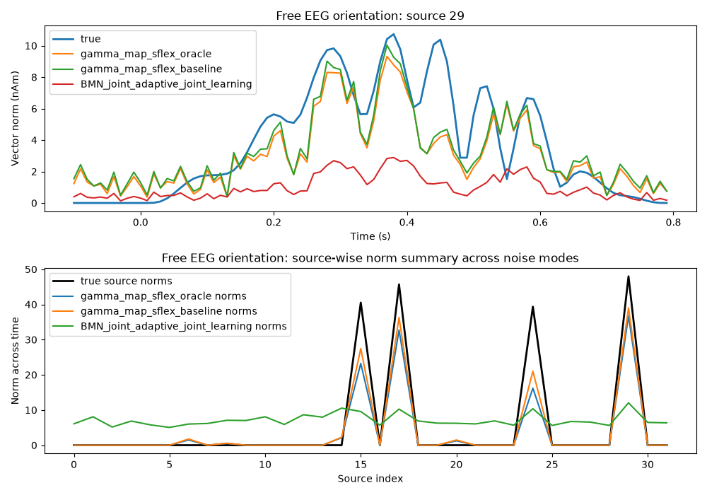
Plot vector norms for one free-orientation source

For free orientation, a source has a 3-component time series. A simple scalar summary is the Euclidean norm across orientation components.

free_source_idx = int(np.atleast_1d(active_free)[0])
true_free_component_norm = np.linalg.norm(x_true_free, axis=1)

fig, axes = plt.subplots(2, 1, figsize=(10, 7), sharex=False)
axes[0].plot(times, true_free_component_norm[free_source_idx], label="true", linewidth=2)
for name, result in free_solver_outputs.items():
    est_norm = np.linalg.norm(result["posterior_mean_reshaped"], axis=1)
    axes[0].plot(times, est_norm[free_source_idx], label=name)
axes[0].set(
    xlabel="Time (s)",
    ylabel="Vector norm (nAm)",
    title=f"Free EEG orientation: source {free_source_idx}",
)
axes[0].legend(loc="best")

axes[1].plot(
    np.arange(n_sources),
    np.linalg.norm(true_free_component_norm, axis=1),
    label="true source norms",
    linewidth=2,
    color="black",
)
for name, result in free_solver_outputs.items():
    est_norm = np.linalg.norm(result["posterior_mean_reshaped"], axis=1)
    axes[1].plot(np.arange(n_sources), np.linalg.norm(est_norm, axis=1), label=f"{name} norms")
axes[1].set(
    xlabel="Source index",
    ylabel="Norm across time",
    title="Free EEG orientation: source-wise norm summary across noise modes",
)
axes[1].legend(loc="best")
fig.tight_layout()

Summary

SourceEstimator is the main reconstruction wrapper used in the current CaliBrain pipeline. It standardizes solver invocation and returns posterior summaries that later feed uncertainty estimation, aggregation, and calibration.

In practice:

• use oracle when the simulated sensor noise is available and you want the matched reference variance;

• use baseline when the noise level should be estimated from the pre-stimulus sensor segment;

• use adaptive_joint_learning when the solver should learn a common noise level jointly from the data;

• pair those modes with gamma_map_sflex, gamma_lambda_map_sflex, BMN, and BMN_joint according to the active workflow config.