00. Motivation

This tutorial introduces the scientific problem addressed by CaliBrain: posterior uncertainty in Bayesian M/EEG source imaging is only useful if its nominal credibility agrees with empirical coverage.

Why uncertainty calibration matters

M/EEG inverse source imaging is an ill-posed problem. Different source configurations can explain similar sensor measurements, so uncertainty is not a secondary detail: it is part of the inference problem itself.

In practice, many inverse workflows focus mainly on reconstructed source activity. CaliBrain asks a more specific question:

• when a solver reports posterior uncertainty,

• do the corresponding credible regions contain the true source activity as often as their nominal coverage suggests?

This question motivates the full CaliBrain workflow:

1. simulate source activity under controlled conditions,

2. project it to sensors through a leadfield,

3. reconstruct posterior means and uncertainty summaries,

4. compare nominal and empirical coverage,

5. optionally recalibrate the nominal coverage levels.

import matplotlib.pyplot as plt
import numpy as np

From point estimates to uncertainty-aware inference

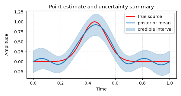
The central distinction is between:

• a point estimate, which summarizes what source activity is believed to be present;

• an uncertainty summary, which quantifies how concentrated or diffuse the posterior distribution is around that estimate.

A useful uncertainty summary should be calibrated: if a nominal 90% credible region is reported repeatedly under comparable conditions, it should contain the true source quantity close to 90% of the time.

time = np.linspace(0.0, 1.0, 200)
true_signal = np.exp(-0.5 * ((time - 0.45) / 0.09) ** 2)
posterior_mean = true_signal + 0.08 * np.sin(8 * np.pi * time)
posterior_std = 0.12 + 0.02 * np.cos(4 * np.pi * time)

fig, ax = plt.subplots(figsize=(6, 3.2))
ax.plot(time, true_signal, color="#ff0000", lw=2, label="true source")
ax.plot(time, posterior_mean, color="#1f77b4", lw=2, label="posterior mean")
ax.fill_between(
    time,
    posterior_mean - 1.96 * posterior_std,
    posterior_mean + 1.96 * posterior_std,
    color="#1f77b4",
    alpha=0.25,
    label="credible interval",
)
ax.set(
    xlabel="Time",
    ylabel="Amplitude",
    title="Point estimate and uncertainty summary",
)
ax.legend(loc="upper right")
ax.grid(True, linestyle="--", alpha=0.4)
fig.tight_layout()

Calibration as agreement between nominal and empirical coverage

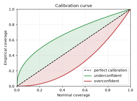
CaliBrain evaluates uncertainty through coverage. For a nominal coverage level \(c\), the empirical coverage measures how often the true source quantity falls inside the corresponding credible region over many source locations or many repeated runs.

Plotting empirical coverage against nominal coverage yields the calibration curve:

• the diagonal corresponds to perfect calibration,

• a curve above the diagonal indicates underconfident uncertainty,

• a curve below the diagonal indicates overconfident uncertainty.

nominal = np.linspace(0.0, 1.0, 200)
underconfident = nominal ** 0.45
overconfident = nominal ** 2.2

fig, ax = plt.subplots(figsize=(5.4, 4.0))
ax.plot(nominal, nominal, "k--", lw=1.5, label="perfect calibration")
ax.plot(nominal, underconfident, color="#55a868", lw=2.2, label="underconfident")
ax.plot(nominal, overconfident, color="#c44e52", lw=2.2, label="overconfident")
ax.fill_between(nominal, nominal, underconfident, color="#55a868", alpha=0.18)
ax.fill_between(nominal, overconfident, nominal, color="#c44e52", alpha=0.18)
ax.set(
    xlabel="Nominal coverage",
    ylabel="Empirical coverage",
    title="Calibration curve",
    xlim=(0, 1),
    ylim=(0, 1),
)
ax.legend(loc="lower right")
ax.grid(True, linestyle="--", alpha=0.35)
fig.tight_layout()

Why CaliBrain distinguishes fixed, free MEG, and free EEG

The same calibration question is studied across three source models:

• fixed orientation,

• free-orientation MEG,

• free-orientation EEG.

These settings differ in the local dimension of the source quantity and therefore in the shape of the associated uncertainty object. Later tutorials turn this into concrete intervals, ellipses, and ellipsoids.

CaliBrain also distinguishes:

• pre-calibration evaluation (precal),

• post-calibration evaluation on matched or pooled training conditions,

• transfer settings such as post_pooled_mismatch and post_fixed.

The underlying recalibration mechanism is the same across these modes; what changes is the choice of training and evaluation splits.

Where to go next

This tutorial motivates the problem. The mathematical formulation is given in Theoretical Foundations.

From there, the practical tutorial sequence continues with:

• Solver Families and Uncertainty Behavior for dense versus sparse solver intuition,

• Quick Start for a minimal coverage example,

• Source Simulation for the synthetic source model,

• Uncertainty Estimation for the uncertainty objects,

• Calibration Methods for recalibration workflows.