10. Calibration Methods

This tutorial explains CaliBrain’s calibration step through the high-level UncertaintyCalibrator API.

All implemented calibration modes use the same recalibration mechanism: isotonic regression on empirical coverage curves. What changes from one mode to another is the train/evaluation split used to fit and test that map.

The tutorial demonstrates:

• precal: evaluate the raw coverage curve without fitting a map;

• post_oracle: fit on a matched training split and evaluate on a matched held-out split.

The remaining modes are then interpreted relative to the same logic: post_pooled, post_pooled_mismatch, and post_fixed.

Scientific motivation

UncertaintyEstimator returns a pre-calibration empirical coverage curve on a nominal grid \(c \in [0, 1]\). If that curve is \(g(c) \neq c\), the posterior uncertainty is miscalibrated.

CaliBrain uses isotonic regression to fit a monotone approximation of \(g(c)\) on training runs and then numerically inverts that fitted curve. The result is a recalibrated nominal coverage grid that is evaluated on a held-out split.

The workflow-level calibration modes used in the documentation are:

• precal: no fit, evaluate raw empirical coverage only;

• post_oracle: fit and evaluate on matched conditions;

• post_pooled: fit on pooled matched conditions and evaluate on one target condition;

• post_pooled_mismatch: fit on intentionally mismatched pooled conditions and evaluate on a target condition;

• post_fixed: fit once at a reference condition and reuse that mapping across a sweep.

These names refer to benchmark-style train/evaluation configurations around a common isotonic recalibration step; they are not five different calibration algorithms.

Just as important: calibration mode does not change the underlying uncertainty representation. Fixed orientation still uses marginal intervals; free orientation still uses either marginal or full_cov depending on the diagnostic being evaluated. Calibration acts on the coverage curve built from those objects; it does not redefine the objects themselves.

import matplotlib.pyplot as plt
import numpy as np
from mne.io.constants import FIFF

from calibrain import (
    MetricEvaluator,
    SensorSimulator,
    SourceEstimator,
    SourceSimulator,
    UncertaintyCalibrator,
    UncertaintyEstimator,
    gamma_map_sflex,
)


RANDOM_SEED = 61

Build a lightweight fixed-orientation calibration fixture

To keep the tutorial executable, we build tiny matched-condition datasets directly in memory. Both train and eval datasets use the same solver, orientation, source coordinates, leadfield shape, and ERP settings. Only the random seed changes.

This corresponds to the conceptual logic of post_oracle: calibration is fitted and evaluated under the same condition family.

erp_config = {
    "tmin": -0.1,
    "tmax": 0.8,
    "stim_onset": 0.0,
    "sfreq": 100,
    "fmin": 2,
    "fmax": 8,
    "amplitude_distribution": {
        "median": 8.0,
        "sigma": 0.15,
        "clip": [2.0, 20.0],
    },
    "random_erp_timing": False,
    "erp_min_length": 20,
}

nominal_coverages = np.linspace(0.0, 1.0, 11)
ue = UncertaintyEstimator(nominal_coverages=nominal_coverages)
me = MetricEvaluator(ue)
source_simulator = SourceSimulator(ERP_config=erp_config)
sensor_simulator = SensorSimulator()

rng = np.random.default_rng(RANDOM_SEED)
n_sensors = 16
n_sources = 32
src_coords = rng.normal(scale=0.04, size=(n_sources, 3))
leadfield_fixed = rng.normal(scale=0.03, size=(n_sensors, n_sources))
leadfield_fixed /= np.maximum(
    np.linalg.norm(leadfield_fixed, axis=0, keepdims=True),
    np.finfo(float).eps,
)
leadfield_fixed *= 0.6

sensor_simulator.set_sensor_metadata(
    kind=FIFF.FIFFV_EEG_CH,
    units=FIFF.FIFF_UNIT_V,
    unitmult=FIFF.FIFF_UNITM_MU,
    coil_type=FIFF.FIFFV_COIL_EEG,
)
x_true_train, _ = source_simulator.simulate(
    n_sources=n_sources,
    nnz=4,
    orientation_type="fixed",
    seed=RANDOM_SEED,
)
y_clean_train, y_noisy_train, noise_train, _ = sensor_simulator.simulate(
    x=x_true_train,
    L=leadfield_fixed,
    alpha_SNR=0.7,
    sensor_white_noise_std=0.2,
    seed=RANDOM_SEED,
)
noise_var_train = float(np.var(noise_train))
estimator_train = SourceEstimator(
    solver=gamma_map_sflex,
    solver_params={"max_iter": 150, "tol": 1e-7, "sigma": 0.01, "src_coords": src_coords},
    noise_var=noise_var_train,
    n_orient=1,
)
estimator_train.fit(leadfield_fixed, y_noisy_train)
result_train = estimator_train.predict()
train_dataset = {
    "orientation_type": "fixed",
    "coil_type": None,
    "x_true": x_true_train,
    "x_hat": result_train["posterior_mean"],
    "posterior_var": ue.posterior_variance_from_cov(result_train["posterior_cov"]),
    "posterior_cov": result_train["posterior_cov"],
    "n_sources": x_true_train.shape[0],
    "n_times": x_true_train.shape[1],
    "noise_var": noise_var_train,
    "alpha_SNR": 0.7,
    "seed": RANDOM_SEED,
    "solver": "gamma_map_sflex",
    "noise_type": "oracle",
}

x_true_eval, _ = source_simulator.simulate(
    n_sources=n_sources,
    nnz=4,
    orientation_type="fixed",
    seed=RANDOM_SEED + 1,
)
y_clean_eval, y_noisy_eval, noise_eval, _ = sensor_simulator.simulate(
    x=x_true_eval,
    L=leadfield_fixed,
    alpha_SNR=0.7,
    sensor_white_noise_std=0.2,
    seed=RANDOM_SEED + 1,
)
noise_var_eval = float(np.var(noise_eval))
estimator_eval = SourceEstimator(
    solver=gamma_map_sflex,
    solver_params={"max_iter": 150, "tol": 1e-7, "sigma": 0.01, "src_coords": src_coords},
    noise_var=noise_var_eval,
    n_orient=1,
)
estimator_eval.fit(leadfield_fixed, y_noisy_eval)
result_eval = estimator_eval.predict()
eval_dataset = {
    "orientation_type": "fixed",
    "coil_type": None,
    "x_true": x_true_eval,
    "x_hat": result_eval["posterior_mean"],
    "posterior_var": ue.posterior_variance_from_cov(result_eval["posterior_cov"]),
    "posterior_cov": result_eval["posterior_cov"],
    "n_sources": x_true_eval.shape[0],
    "n_times": x_true_eval.shape[1],
    "noise_var": noise_var_eval,
    "alpha_SNR": 0.7,
    "seed": RANDOM_SEED + 1,
    "solver": "gamma_map_sflex",
    "noise_type": "oracle",
}

print("train dataset keys:", sorted(train_dataset.keys()))
print("eval dataset keys:", sorted(eval_dataset.keys()))
print("train posterior_var shape:", train_dataset["posterior_var"].shape)
print("eval posterior_var shape:", eval_dataset["posterior_var"].shape)

train dataset keys: ['alpha_SNR', 'coil_type', 'n_sources', 'n_times', 'noise_type', 'noise_var', 'orientation_type', 'posterior_cov', 'posterior_var', 'seed', 'solver', 'x_hat', 'x_true']
eval dataset keys: ['alpha_SNR', 'coil_type', 'n_sources', 'n_times', 'noise_type', 'noise_var', 'orientation_type', 'posterior_cov', 'posterior_var', 'seed', 'solver', 'x_hat', 'x_true']
train posterior_var shape: (32,)
eval posterior_var shape: (32,)

Mode 1: precal

precal means: do not fit a recalibration map. Evaluate the raw empirical coverage on the evaluation split only. In the class API, this is fit=False.

precal_calibrator = UncertaintyCalibrator(ue, me)
precal_results = precal_calibrator.calibrate(
    test_data=eval_dataset,
    fit=False,
)

print("precal nominal coverages:", precal_results["pre_calibration"]["nominal_coverages"])
print("precal empirical coverages:", precal_results["pre_calibration"]["empirical_coverages"])
print("precal post block equals pre block:", np.allclose(
    precal_results["pre_calibration"]["empirical_coverages"],
    precal_results["post_calibration"]["empirical_coverages"],
))
print("precal recalibrated nominal coverages:", precal_results["post_calibration"]["recalibrated_nominal_coverages"])

precal nominal coverages: [0.  0.1 0.2 0.3 0.4 0.5 0.6 0.7 0.8 0.9 1. ]
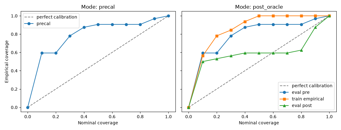
precal empirical coverages: [0.      0.59375 0.59375 0.78125 0.875   0.90625 0.90625 0.90625 0.90625
 0.96875 1.     ]
precal post block equals pre block: True
precal recalibrated nominal coverages: [0.  0.1 0.2 0.3 0.4 0.5 0.6 0.7 0.8 0.9 1. ]

Mode 2: post_oracle

post_oracle means: fit a recalibration map on a matched train split and evaluate it on a matched eval split. In the class API, this is the same high-level method, but now with train_data, test_data, and fit=True.

post_oracle_calibrator = UncertaintyCalibrator(ue, me)
post_oracle_results = post_oracle_calibrator.calibrate(
    train_data=train_dataset,
    test_data=eval_dataset,
    fit=True,
)

print("post_oracle train empirical coverages:", post_oracle_results["train_empirical_coverages"])
print("post_oracle pre empirical coverages:", post_oracle_results["pre_calibration"]["empirical_coverages"])
print("post_oracle post empirical coverages:", post_oracle_results["post_calibration"]["empirical_coverages"])
print("post_oracle recalibrated nominal coverages:", post_oracle_results["post_calibration"]["recalibrated_nominal_coverages"])

post_oracle train empirical coverages: [0.      0.5625  0.78125 0.84375 0.9375  1.      1.      1.      1.
 1.      1.     ]
post_oracle pre empirical coverages: [0.      0.59375 0.59375 0.78125 0.875   0.90625 0.90625 0.90625 0.90625
 0.96875 1.     ]
post_oracle post empirical coverages: [0.      0.5     0.53125 0.5625  0.59375 0.59375 0.59375 0.59375 0.625
 0.875   1.     ]
post_oracle recalibrated nominal coverages: [0.         0.01777778 0.03555556 0.05333333 0.07111111 0.08888889
 0.11714286 0.16285714 0.23       0.36       1.        ]

Inspect the learned recalibration map

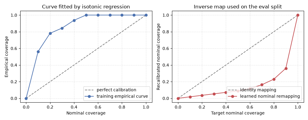
The fitted isotonic model is learned on the training empirical curve. The returned recalibrated_nominal_coverages are the inverse-mapped nominal levels used when the evaluation split is rechecked after calibration.

fig, axes = plt.subplots(1, 2, figsize=(10.2, 4.0))

axes[0].plot([0, 1], [0, 1], "--", color="0.5", label="perfect calibration")
axes[0].plot(
    post_oracle_results["pre_calibration"]["nominal_coverages"],
    post_oracle_results["train_empirical_coverages"],
    "o-",
    color="#4c72b0",
    label="training empirical curve",
)
axes[0].set(
    xlabel="Nominal coverage",
    ylabel="Empirical coverage",
    title="Curve fitted by isotonic regression",
)
axes[0].legend(loc="lower right")
axes[0].grid(True, linestyle="--", alpha=0.35)

axes[1].plot([0, 1], [0, 1], "--", color="0.5", label="identity mapping")
axes[1].plot(
    post_oracle_results["post_calibration"]["nominal_coverages"],
    post_oracle_results["post_calibration"]["recalibrated_nominal_coverages"],
    "o-",
    color="#c44e52",
    label="learned nominal remapping",
)
axes[1].set(
    xlabel="Target nominal coverage",
    ylabel="Recalibrated nominal coverage",
    title="Inverse map used on the eval split",
)
axes[1].legend(loc="lower right")
axes[1].grid(True, linestyle="--", alpha=0.35)

fig.tight_layout()

The other workflow modes

The remaining modes differ only in how the workflow constructs train_data and test_data:

• post_pooled: pool several matched training conditions before fitting one map;

• post_pooled_mismatch: fit on pooled training conditions that intentionally differ from the target evaluation condition;

• post_fixed: fit one reference map once and reuse it across a parameter sweep.

In all three cases:

• the uncertainty representation is unchanged;

• the same isotonic-regression mechanism is used;

• only the split logic changes.

This is what lets the workflows study recalibration transfer across conditions rather than mixing up transfer effects with a different calibration algorithm. Broader evaluation choices are covered in Metric Evaluation.

Plot precal and post_oracle

The first panel shows raw pre-calibration coverage. The second panel compares the matched post-calibration result against the raw eval curve and the training empirical curve used to fit the isotonic map.

fig, axes = plt.subplots(1, 2, figsize=(11, 4.2), sharey=True)

axes[0].plot([0, 1], [0, 1], "--", color="0.5", label="perfect calibration")
axes[0].plot(
    precal_results["pre_calibration"]["nominal_coverages"],
    precal_results["pre_calibration"]["empirical_coverages"],
    marker="o",
    label="precal",
)
axes[0].set(
    xlabel="Nominal coverage",
    ylabel="Empirical coverage",
    title="Mode: precal",
)
axes[0].legend(loc="best")

axes[1].plot([0, 1], [0, 1], "--", color="0.5", label="perfect calibration")
axes[1].plot(
    post_oracle_results["pre_calibration"]["nominal_coverages"],
    post_oracle_results["pre_calibration"]["empirical_coverages"],
    marker="o",
    label="eval pre",
)
axes[1].plot(
    post_oracle_results["pre_calibration"]["nominal_coverages"],
    post_oracle_results["train_empirical_coverages"],
    marker="s",
    label="train empirical",
)
axes[1].plot(
    post_oracle_results["post_calibration"]["nominal_coverages"],
    post_oracle_results["post_calibration"]["empirical_coverages"],
    marker="^",
    label="eval post",
)
axes[1].set(
    xlabel="Nominal coverage",
    title="Mode: post_oracle",
)
axes[1].legend(loc="best")

fig.tight_layout()

Inspect metric summaries

UncertaintyCalibrator also returns the default calibration metrics from MetricEvaluator for both the pre- and post-calibration curves.

print("precal metrics:", precal_results["pre_calibration"]["calibration_metrics"])
print("post_oracle pre metrics:", post_oracle_results["pre_calibration"]["calibration_metrics"])
print("post_oracle post metrics:", post_oracle_results["post_calibration"]["calibration_metrics"])

precal metrics: {'max_underconfidence_deviation': 0.0, 'max_overconfidence_deviation': 0.49375, 'mean_absolute_deviation': 0.26704545454545453, 'mean_signed_deviation': 0.26704545454545453}
post_oracle pre metrics: {'max_underconfidence_deviation': 0.0, 'max_overconfidence_deviation': 0.49375, 'mean_absolute_deviation': 0.26704545454545453, 'mean_signed_deviation': 0.26704545454545453}
post_oracle post metrics: {'max_underconfidence_deviation': 0.17500000000000004, 'max_overconfidence_deviation': 0.4, 'mean_absolute_deviation': 0.14488636363636367, 'mean_signed_deviation': 0.08806818181818178}

Summary

UncertaintyCalibrator is the high-level API that realizes CaliBrain’s calibration modes.

In this tutorial:

• precal evaluated raw empirical coverage without fitting a map;

• post_oracle fitted isotonic recalibration on a matched train split and evaluated the recalibrated curve on a matched eval split;

• the learned map was inspected both as a fitted training curve and as an inverse nominal remapping;

• post_pooled, post_pooled_mismatch, and post_fixed were explained as workflow-level variations in how the train/eval splits are constructed.