
Note
Go to the end to download the full example code.
12. End-to-End Workflow#
This tutorial ties together the main CaliBrain component classes in one small, runnable workflow:
SourceSimulatorfor source-level ground truth;LeadfieldBuilderfor a leadfield object;SensorSimulatorfor noisy sensor measurements;SourceEstimatorfor posterior source reconstruction;UncertaintyEstimatorfor pre-calibration empirical coverage;UncertaintyCalibratorfor post-calibration isotonic recalibration.
It is intentionally lightweight and fully synthetic, but it follows the same scientific order as the current fixed-orientation calibration workflow: simulation, inversion, uncertainty representation, and calibration.
Scientific motivation#
CaliBrain studies whether posterior uncertainty from inverse source imaging is empirically calibrated. An end-to-end run therefore needs all upstream pieces that define the coverage curve:
simulate source activity
x_true;obtain a leadfield
L;project to noisy sensors
y_noisy;reconstruct posterior mean and covariance;
derive an uncertainty representation and empirical coverage;
fit a recalibration map on a train split and evaluate it on a held-out split.
This tutorial demonstrates that full chain with the current high-level class
interfaces and an active fixed-orientation solver. The concrete example below
follows the logic of post_oracle. Other documented workflow examples such
as post_pooled, post_pooled_mismatch, and post_fixed change the
split construction, not the underlying recalibration mechanism. Evaluation can
then be extended beyond this one example with the tools shown in
Metric Evaluation.
import matplotlib.pyplot as plt
import numpy as np
from mne.io.constants import FIFF

from calibrain import (
    LeadfieldBuilder,
    MetricEvaluator,
    SensorSimulator,
    SourceEstimator,
    SourceSimulator,
    UncertaintyCalibrator,
    UncertaintyEstimator,
    gamma_map_sflex,
)


RANDOM_SEED = 91

# Step 1: define a compact fixed-orientation simulation setting
# -------------------------------------------------------------
#
# We keep the example fixed-orientation because it is the smallest configuration
# that still exercises the full calibration chain. The same scientific logic
# extends to free orientation in later tutorials.

erp_config = {
    "tmin": -0.1,
    "tmax": 0.8,
    "stim_onset": 0.0,
    "sfreq": 100,
    "fmin": 2,
    "fmax": 8,
    "amplitude_distribution": {
        "median": 8.0,
        "sigma": 0.15,
        "clip": [2.0, 20.0],
    },
    "random_erp_timing": False,
    "erp_min_length": 20,
}

n_sensors = 16
n_sources = 32
nnz = 4
alpha_snr = 0.7
nominal_coverages = np.linspace(0.0, 1.0, 11)

source_simulator = SourceSimulator(ERP_config=erp_config)
sensor_simulator = SensorSimulator()
uncertainty_estimator = UncertaintyEstimator(nominal_coverages=nominal_coverages)
metric_evaluator = MetricEvaluator(uncertainty_estimator)

sensor_simulator.set_sensor_metadata(
    kind=FIFF.FIFFV_EEG_CH,
    units=FIFF.FIFF_UNIT_V,
    unitmult=FIFF.FIFF_UNITM_MU,
    coil_type=FIFF.FIFFV_COIL_EEG,
)
Step 2: build a deterministic synthetic leadfield#
In larger simulation studies, LeadfieldBuilder usually loads a
precomputed subject-specific leadfield. Here we use its lightweight
random mode and pair it with synthetic source coordinates for the sFLEX
solver.
leadfield_builder = LeadfieldBuilder(leadfield_dir="unused_demo_leadfields")
leadfield_data = leadfield_builder.get_leadfield(
    subject="demo",
    orientation_type="fixed",
    retrieve_mode="random",
    n_sensors=n_sensors,
    n_sources=n_sources,
    return_metadata=True,
)

L = leadfield_data.leadfield
src_coords = np.random.default_rng(RANDOM_SEED).normal(scale=0.04, size=(n_sources, 3))

print("leadfield shape:", L.shape)
print("source coordinates shape:", src_coords.shape)
leadfield shape: (16, 32)
source coordinates shape: (32, 3)
Step 3: generate matched train/eval datasets#
A calibration tutorial needs at least two splits:
a train split for fitting the isotonic recalibration map;
an eval split for reporting pre- and post-calibration coverage.
We keep the condition family fixed and change only the random seed. This
corresponds to the logic of post_oracle in the workflow documentation.
x_true_train, active_sources_train = source_simulator.simulate(
    n_sources=n_sources,
    nnz=nnz,
    orientation_type="fixed",
    seed=RANDOM_SEED,
)
y_clean_train, y_noisy_train, noise_train, _ = sensor_simulator.simulate(
    x=x_true_train,
    L=L,
    alpha_SNR=alpha_snr,
    sensor_white_noise_std=0.2,
    seed=RANDOM_SEED,
)
noise_var_train = max(float(np.var(noise_train)), 1e-12)
estimator_train = SourceEstimator(
    solver=gamma_map_sflex,
    solver_params={"max_iter": 150, "tol": 1e-7, "sigma": 0.01, "src_coords": src_coords},
    noise_var=noise_var_train,
    n_orient=1,
)
estimator_train.fit(L, y_noisy_train)
result_train = estimator_train.predict()
train_dataset = {
    "orientation_type": "fixed",
    "coil_type": None,
    "x_true": x_true_train,
    "x_hat": result_train["posterior_mean"],
    "posterior_cov": result_train["posterior_cov"],
    "posterior_var": uncertainty_estimator.posterior_variance_from_cov(result_train["posterior_cov"]),
    "n_sources": x_true_train.shape[0],
    "n_times": x_true_train.shape[1],
    "seed": RANDOM_SEED,
    "nnz": nnz,
    "alpha_SNR": alpha_snr,
    "solver": "gamma_map_sflex",
    "noise_type": "oracle",
    "active_sources": active_sources_train,
    "noise_var": noise_var_train,
}

x_true_eval, active_sources_eval = source_simulator.simulate(
    n_sources=n_sources,
    nnz=nnz,
    orientation_type="fixed",
    seed=RANDOM_SEED + 1,
)
y_clean_eval, y_noisy_eval, noise_eval, _ = sensor_simulator.simulate(
    x=x_true_eval,
    L=L,
    alpha_SNR=alpha_snr,
    sensor_white_noise_std=0.2,
    seed=RANDOM_SEED + 1,
)
noise_var_eval = max(float(np.var(noise_eval)), 1e-12)
estimator_eval = SourceEstimator(
    solver=gamma_map_sflex,
    solver_params={"max_iter": 150, "tol": 1e-7, "sigma": 0.01, "src_coords": src_coords},
    noise_var=noise_var_eval,
    n_orient=1,
)
estimator_eval.fit(L, y_noisy_eval)
result_eval = estimator_eval.predict()
eval_dataset = {
    "orientation_type": "fixed",
    "coil_type": None,
    "x_true": x_true_eval,
    "x_hat": result_eval["posterior_mean"],
    "posterior_cov": result_eval["posterior_cov"],
    "posterior_var": uncertainty_estimator.posterior_variance_from_cov(result_eval["posterior_cov"]),
    "n_sources": x_true_eval.shape[0],
    "n_times": x_true_eval.shape[1],
    "seed": RANDOM_SEED + 1,
    "nnz": nnz,
    "alpha_SNR": alpha_snr,
    "solver": "gamma_map_sflex",
    "noise_type": "oracle",
    "active_sources": active_sources_eval,
    "noise_var": noise_var_eval,
}

print("train x_true shape:", train_dataset["x_true"].shape)
print("eval x_hat shape:", eval_dataset["x_hat"].shape)
print("eval posterior_var shape:", eval_dataset["posterior_var"].shape)
train x_true shape: (32, 90)
eval x_hat shape: (32, 90)
eval posterior_var shape: (32,)
Step 4: compute the pre-calibration coverage curve#
UncertaintyEstimator converts posterior means and source-wise variances
into intervals over the nominal coverage grid. In the current workflow,
calibration is typically performed in aggregated mode, so we use the
time-aggregated interval routine here.
pre_curve = uncertainty_estimator.calibration_curve_intervals_aggregated(
    x_true=eval_dataset["x_true"],
    x_hat=eval_dataset["x_hat"],
    posterior_var=eval_dataset["posterior_var"],
)
pre_metrics = metric_evaluator.calibration_metrics_4(
    pre_curve["nominal_coverages"],
    pre_curve["empirical_coverages"],
)

print("pre empirical coverages:", np.round(pre_curve["empirical_coverages"], 3))
print("pre calibration metrics:", pre_metrics)
pre empirical coverages: [0.    0.438 0.5   0.594 0.656 0.688 0.719 0.75  0.875 0.938 1.   ]
pre calibration metrics: {'max_underconfidence_deviation': 0.0, 'max_overconfidence_deviation': 0.3375, 'mean_absolute_deviation': 0.15056818181818177, 'mean_signed_deviation': 0.15056818181818177}
Step 5: fit and evaluate post-calibration#
UncertaintyCalibrator consumes the same dataset structure used by the
workflow. Here we fit on the train split and evaluate on the matched eval
split. This is the high-level class API corresponding to post_oracle.
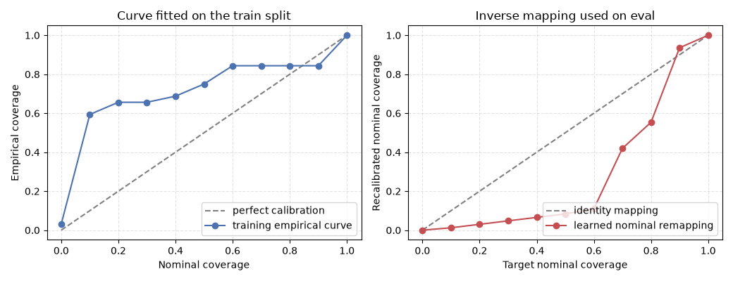
The crucial point is that calibration changes the nominal coverage values used to build intervals on the evaluation split. It does not change the posterior mean, posterior covariance, or uncertainty type.
calibrator = UncertaintyCalibrator(uncertainty_estimator, metric_evaluator)
calibration_result = calibrator.calibrate(
    train_data=train_dataset,
    test_data=eval_dataset,
    fit=True,
)

post_block = calibration_result["post_calibration"]
print(
    "post recalibrated nominal coverages:",
    np.round(post_block["recalibrated_nominal_coverages"], 3),
)
print(
    "post empirical coverages:",
    np.round(post_block["empirical_coverages"], 3),
)
post recalibrated nominal coverages: [0.    0.012 0.03  0.048 0.066 0.083 0.11  0.42  0.553 0.936 1.   ]
post empirical coverages: [0.    0.188 0.281 0.344 0.375 0.406 0.438 0.688 0.719 0.969 1.   ]
Step 6: inspect the learned recalibration map#
The training empirical curve is what isotonic regression fits. The learned inverse map is then used to choose recalibrated nominal levels on the held-out split.
fig, axes = plt.subplots(1, 2, figsize=(10.4, 4.0))

axes[0].plot([0, 1], [0, 1], "--", color="0.5", label="perfect calibration")
axes[0].plot(
    pre_curve["nominal_coverages"],
    calibration_result["train_empirical_coverages"],
    "o-",
    color="#4c72b0",
    label="training empirical curve",
)
axes[0].set(
    xlabel="Nominal coverage",
    ylabel="Empirical coverage",
    title="Curve fitted on the train split",
)
axes[0].legend(loc="lower right")
axes[0].grid(True, linestyle="--", alpha=0.35)

axes[1].plot([0, 1], [0, 1], "--", color="0.5", label="identity mapping")
axes[1].plot(
    post_block["nominal_coverages"],
    post_block["recalibrated_nominal_coverages"],
    "o-",
    color="#c44e52",
    label="learned nominal remapping",
)
axes[1].set(
    xlabel="Target nominal coverage",
    ylabel="Recalibrated nominal coverage",
    title="Inverse mapping used on eval",
)
axes[1].legend(loc="lower right")
axes[1].grid(True, linestyle="--", alpha=0.35)

fig.tight_layout()
Step 9: visualize the full end-to-end result#
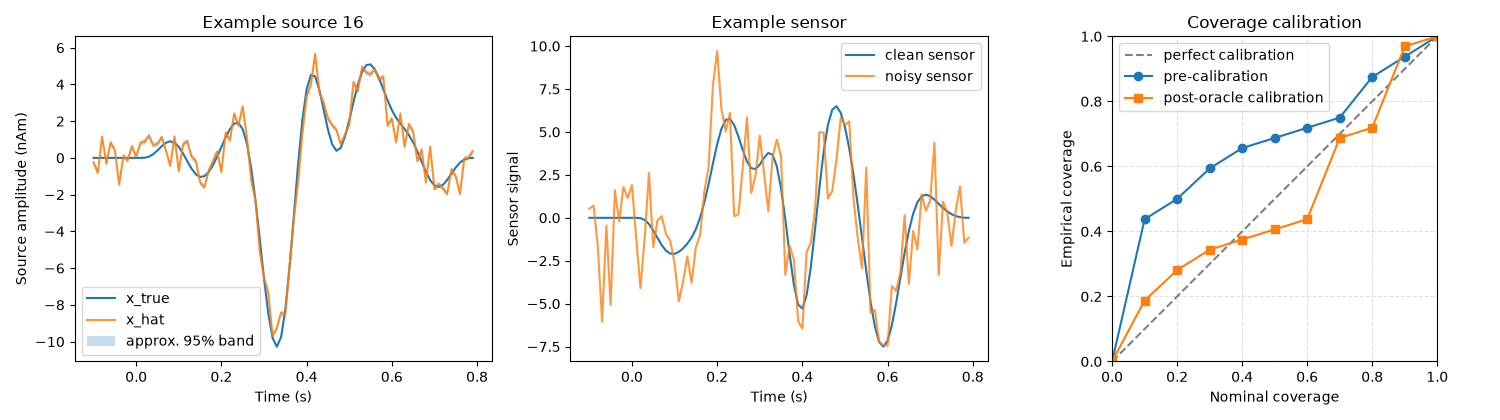
The figure summarizes three stages of the workflow:
one reconstructed source waveform;
one clean/noisy sensor trace;
pre- and post-calibration coverage curves.
time = np.arange(train_dataset["x_true"].shape[1]) / erp_config["sfreq"] + erp_config["tmin"]
example_source = int(eval_dataset["active_sources"][0])

fig, axes = plt.subplots(1, 3, figsize=(15, 4.2))

axes[0].plot(time, eval_dataset["x_true"][example_source], label="x_true")
axes[0].plot(time, eval_dataset["x_hat"][example_source], label="x_hat", alpha=0.85)
band = 1.96 * np.sqrt(eval_dataset["posterior_var"][example_source] / eval_dataset["x_true"].shape[1])
axes[0].fill_between(
    time,
    eval_dataset["x_hat"][example_source] - band,
    eval_dataset["x_hat"][example_source] + band,
    alpha=0.25,
    label="approx. 95% band",
)
axes[0].set(
    xlabel="Time (s)",
    ylabel="Source amplitude (nAm)",
    title=f"Example source {example_source}",
)
axes[0].legend(loc="best")

y_clean_eval, y_noisy_eval, _, _ = sensor_simulator.simulate(
    x=eval_dataset["x_true"],
    L=L,
    alpha_SNR=alpha_snr,
    sensor_white_noise_std=0.2,
    seed=int(eval_dataset["seed"]),
)

axes[1].plot(time, y_clean_eval[0], label="clean sensor")
axes[1].plot(time, y_noisy_eval[0], label="noisy sensor", alpha=0.8)
axes[1].set(
    xlabel="Time (s)",
    ylabel="Sensor signal",
    title="Example sensor",
)
axes[1].legend(loc="best")

axes[2].plot([0, 1], [0, 1], "--", color="0.5", label="perfect calibration")
axes[2].plot(
    pre_curve["nominal_coverages"],
    pre_curve["empirical_coverages"],
    "o-",
    label="pre-calibration",
)
axes[2].plot(
    post_block["nominal_coverages"],
    post_block["empirical_coverages"],
    "s-",
    label="post-oracle calibration",
)
axes[2].set(
    xlabel="Nominal coverage",
    ylabel="Empirical coverage",
    xlim=(0, 1),
    ylim=(0, 1),
    title="Coverage calibration",
)
axes[2].set_aspect("equal", adjustable="box")
axes[2].grid(True, linestyle="--", alpha=0.4)
axes[2].legend(loc="best")

fig.tight_layout()
Summary#
This single tutorial used the current high-level component interfaces in the same order as the calibration workflow:
SourceSimulatorproduced ground-truth source activity;LeadfieldBuildersupplied a leadfield and source coordinates;SensorSimulatorgenerated noisy sensor measurements;SourceEstimatorproduced posterior means and covariance;UncertaintyEstimatorturned that posterior summary into an aggregated interval-based coverage curve;UncertaintyCalibratorfitted and evaluated an isotonic recalibration mapping on matched train/eval splits.
The same sequence underlies the larger workflow scripts. What changes there is scale and split construction, not the scientific role of each stage.
Total running time of the script: (0 minutes 0.605 seconds)