
Note
Go to the end to download the full example code.
08. Source Estimation#
This tutorial explains the SourceEstimator class.
It demonstrates the current CaliBrain source-estimation interface using the active inverse solvers that are part of the pipeline:
gamma_map_sflexfor sparse Bayesian estimation with an sFLEX basis;gamma_lambda_map_sflexfor the sFLEX variant with joint noise learning;BMNfor Bayesian minimum-norm estimation with fixed noise variance;BMN_jointfor Bayesian minimum-norm estimation with joint noise learning.
The examples cover:
fixed-orientation source estimation;
comparison of sparse and minimum-norm posterior summaries;
free-orientation EEG source estimation with a 3-component leadfield;
explicit use of the workflow noise modes
oracle,baseline, andadaptive_joint_learning.
Scientific motivation#
SourceEstimator is the stage that converts sensor data and a leadfield
into posterior source summaries. In CaliBrain, that stage does not stand on
its own: its outputs are passed directly to uncertainty estimation and then to
calibration.
The important outputs are:
posterior_mean: reconstructed source time courses;posterior_cov: posterior covariance in coefficient space;solver-specific diagnostics such as active sets, learned hyperparameters, or learned noise levels.
This means source estimation is not only about recovering a signal. It also determines the uncertainty object that downstream tutorials will evaluate.
import matplotlib.pyplot as plt
import numpy as np
from mne.io.constants import FIFF

from calibrain import (
    BMN,
    BMN_joint,
    SensorSimulator,
    SourceEstimator,
    SourceSimulator,
    gamma_lambda_map_sflex,
    gamma_map_sflex,
)


RANDOM_SEED = 41

# Build a lightweight simulation setup
# ------------------------------------
#
# The source simulator generates sparse ERP-like activity. We then construct
# small synthetic EEG leadfields so the tutorial runs quickly during docs
# builds.
#
# The parameter meanings are the same as in the source-simulation tutorial:
#
# - ``tmin`` and ``tmax`` define the simulated time window in seconds;
# - ``stim_onset`` marks the ERP onset;
# - ``sfreq`` is the sampling frequency in Hz;
# - ``amplitude_distribution`` controls source amplitudes in ``nAm``.
#
# For the sFLEX solvers we also need source coordinates. Here they are small
# synthetic positions in meters. ``sigma=0.01`` therefore means a spatial scale
# of ``10 mm``.
#
# In this tutorial:
#
# - the synthetic EEG leadfield is interpreted in ``µV / nAm``;
# - the simulated sensor data are therefore in ``µV``;
# - posterior means stay in source-amplitude units, i.e. ``nAm``.

erp_config = {
    "tmin": -0.1,
    "tmax": 0.8,
    "stim_onset": 0.0,
    "sfreq": 100,
    "fmin": 2,
    "fmax": 8,
    "amplitude_distribution": {
        "median": 8.0,
        "sigma": 0.15,
        "clip": [2.0, 20.0],
    },
    "random_erp_timing": False,
    "erp_min_length": 20,
}

times = np.arange(erp_config["tmin"], erp_config["tmax"], 1.0 / erp_config["sfreq"])
source_simulator = SourceSimulator(ERP_config=erp_config)
sensor_simulator = SensorSimulator()

rng = np.random.default_rng(RANDOM_SEED)
n_sensors = 16
n_sources = 32
src_coords = rng.normal(scale=0.04, size=(n_sources, 3))

leadfield_fixed = rng.normal(scale=0.03, size=(n_sensors, n_sources))
leadfield_fixed /= np.maximum(
    np.linalg.norm(leadfield_fixed, axis=0, keepdims=True),
    np.finfo(float).eps,
)
leadfield_fixed *= 0.6

leadfield_free_eeg = rng.normal(scale=0.015, size=(n_sensors, n_sources, 3))
leadfield_free_eeg /= np.maximum(
    np.linalg.norm(leadfield_free_eeg, axis=0, keepdims=True),
    np.finfo(float).eps,
)
leadfield_free_eeg *= 0.4

sensor_simulator.set_sensor_metadata(
    kind=FIFF.FIFFV_EEG_CH,
    units=FIFF.FIFF_UNIT_V,
    unitmult=FIFF.FIFF_UNITM_MU,
    coil_type=FIFF.FIFFV_COIL_EEG,
)
Fixed-orientation example#
Fixed orientation uses one coefficient per source, so the leadfield has shape
(n_sensors, n_sources) and the posterior mean has shape
(n_sources, n_times).
x_true_fixed, active_fixed = source_simulator.simulate(
    n_sources=n_sources,
    nnz=4,
    orientation_type="fixed",
    seed=RANDOM_SEED,
)

y_fixed_clean, y_fixed_noisy, fixed_noise, fixed_eta = sensor_simulator.simulate(
    x=x_true_fixed,
    L=leadfield_fixed,
    alpha_SNR=0.7,
    sensor_white_noise_std=0.2,
    seed=RANDOM_SEED,
)

tmin = erp_config["tmin"]
stim_onset = erp_config["stim_onset"]
sfreq = erp_config["sfreq"]
pre_stimulus_onset = int((stim_onset - tmin) * sfreq)
y_fixed_pre = y_fixed_noisy[:, :pre_stimulus_onset]

oracle_noise_var = float(np.var(fixed_noise))
baseline_noise_var = float(np.mean(np.std(y_fixed_pre, axis=1) ** 2))

print("fixed source shape:", x_true_fixed.shape)
print("fixed sensor shape:", y_fixed_noisy.shape)
print("fixed active sources:", active_fixed)
print("fixed eta:", fixed_eta)
print("oracle noise variance:", oracle_noise_var)
print("baseline noise variance:", baseline_noise_var)
print("adaptive joint learning noise variance:", None)
fixed source shape: (32, 90)
fixed sensor shape: (16, 90)
fixed active sources: [11 31 10 24]
fixed eta: 1.82281324753165
oracle noise variance: 0.1397447217185092
baseline noise variance: 0.11194502692152937
adaptive joint learning noise variance: None
Fixed orientation: compare solver families and noise modes#
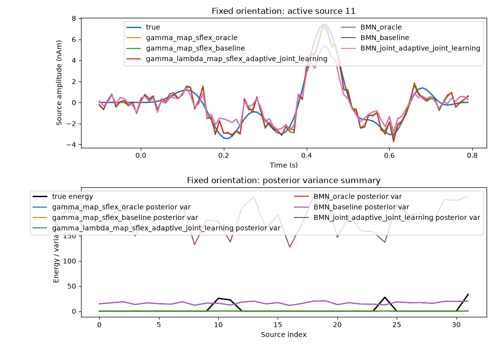
The sparse gamma-MAP family and the dense minimum-norm family can produce different posterior structures even when fitted to the same data. This is one reason why later uncertainty and calibration behavior can differ by solver.
solver_outputs = {}
solver_specs = [
    (
        "gamma_map_sflex_oracle",
        gamma_map_sflex,
        {"max_iter": 150, "tol": 1e-7, "sigma": 0.01, "src_coords": src_coords},
        oracle_noise_var,
    ),
    (
        "gamma_map_sflex_baseline",
        gamma_map_sflex,
        {"max_iter": 150, "tol": 1e-7, "sigma": 0.01, "src_coords": src_coords},
        baseline_noise_var,
    ),
    (
        "gamma_lambda_map_sflex_adaptive_joint_learning",
        gamma_lambda_map_sflex,
        {
            "max_iter": 150,
            "tol": 1e-7,
            "sigma": 0.01,
            "src_coords": src_coords,
            "learn_lambda": True,
        },
        None,
    ),
    (
        "BMN_oracle",
        BMN,
        {"max_iter": 300, "tol": 1e-7, "normalization": False},
        oracle_noise_var,
    ),
    (
        "BMN_baseline",
        BMN,
        {"max_iter": 300, "tol": 1e-7, "normalization": False},
        baseline_noise_var,
    ),
    (
        "BMN_joint_adaptive_joint_learning",
        BMN_joint,
        {"max_iter": 300, "tol": 1e-7, "normalization": False, "learn_noise": True},
        None,
    ),
]

for name, solver, solver_params, noise_var in solver_specs:
    estimator = SourceEstimator(
        solver=solver,
        solver_params=solver_params,
        noise_var=noise_var,
        n_orient=1,
    )
    estimator.fit(leadfield_fixed, y_fixed_noisy)
    solver_outputs[name] = estimator.predict()

for name, result in solver_outputs.items():
    print(f"{name} result keys:", sorted(result.keys()))
    print(f"{name} posterior_mean shape:", result["posterior_mean"].shape)
    print(f"{name} posterior_cov shape:", result["posterior_cov"].shape)
    print(f"{name} learned or used noise_var:", result.get("noise_var"))
gamma_map_sflex_oracle result keys: ['B_spatial', 'active_indices', 'active_source_indices', 'coefficient_indices', 'gamma', 'gammas_full', 'n_iter', 'n_orient', 'noise_var', 'posterior_cov', 'posterior_cov_coeff', 'posterior_mean', 'posterior_mean_coeff', 'source_indices']
gamma_map_sflex_oracle posterior_mean shape: (32, 90)
gamma_map_sflex_oracle posterior_cov shape: (32, 32)
gamma_map_sflex_oracle learned or used noise_var: 0.1397447217185092
gamma_map_sflex_baseline result keys: ['B_spatial', 'active_indices', 'active_source_indices', 'coefficient_indices', 'gamma', 'gammas_full', 'n_iter', 'n_orient', 'noise_var', 'posterior_cov', 'posterior_cov_coeff', 'posterior_mean', 'posterior_mean_coeff', 'source_indices']
gamma_map_sflex_baseline posterior_mean shape: (32, 90)
gamma_map_sflex_baseline posterior_cov shape: (32, 32)
gamma_map_sflex_baseline learned or used noise_var: 0.11194502692152937
gamma_lambda_map_sflex_adaptive_joint_learning result keys: ['B_operator', 'active_indices', 'coefficient_indices', 'err_gamma_hist', 'gamma', 'gammas_full', 'lambda_mean', 'lambda_mean_hist', 'lambdas', 'n_active_hist', 'noise_var', 'posterior_cov', 'posterior_cov_active', 'posterior_cov_active_coeff', 'posterior_cov_coeff', 'posterior_mean', 'posterior_mean_coeff', 'source_indices']
gamma_lambda_map_sflex_adaptive_joint_learning posterior_mean shape: (32, 90)
gamma_lambda_map_sflex_adaptive_joint_learning posterior_cov shape: (32, 32)
gamma_lambda_map_sflex_adaptive_joint_learning learned or used noise_var: 0.11186522283608982
BMN_oracle result keys: ['active_indices', 'coefficient_indices', 'gamma', 'noise_var', 'posterior_cov', 'posterior_mean', 'source_indices']
BMN_oracle posterior_mean shape: (32, 90)
BMN_oracle posterior_cov shape: (32, 32)
BMN_oracle learned or used noise_var: 0.1397447217185092
BMN_baseline result keys: ['active_indices', 'coefficient_indices', 'gamma', 'noise_var', 'posterior_cov', 'posterior_mean', 'source_indices']
BMN_baseline posterior_mean shape: (32, 90)
BMN_baseline posterior_cov shape: (32, 32)
BMN_baseline learned or used noise_var: 0.11194502692152937
BMN_joint_adaptive_joint_learning result keys: ['active_indices', 'coefficient_indices', 'err_gamma_hist', 'gamma', 'gamma_hist', 'lambda', 'lambda_hist', 'noise_var', 'noise_var_hist', 'posterior_cov', 'posterior_mean', 'source_indices']
BMN_joint_adaptive_joint_learning posterior_mean shape: (32, 90)
BMN_joint_adaptive_joint_learning posterior_cov shape: (32, 32)
BMN_joint_adaptive_joint_learning learned or used noise_var: 2.904477730519163e-13
Inspect fixed-orientation posterior summaries#
A useful first check is whether the reconstructed activity on a true active source follows the simulated ERP, and how the source-wise posterior variance differs across solver families and noise modes.
fixed_source_idx = int(np.atleast_1d(active_fixed)[0])
source_energy_true = np.linalg.norm(x_true_fixed, axis=1)
source_axis = np.arange(n_sources)
plot_order = [
    "gamma_map_sflex_oracle",
    "gamma_map_sflex_baseline",
    "gamma_lambda_map_sflex_adaptive_joint_learning",
    "BMN_oracle",
    "BMN_baseline",
    "BMN_joint_adaptive_joint_learning",
]

fig, axes = plt.subplots(2, 1, figsize=(10, 7), sharex=False)
axes[0].plot(times, x_true_fixed[fixed_source_idx], label="true", linewidth=2)
for name in plot_order:
    axes[0].plot(times, solver_outputs[name]["posterior_mean"][fixed_source_idx], label=name)
axes[0].set(
    xlabel="Time (s)",
    ylabel="Source amplitude (nAm)",
    title=f"Fixed orientation: active source {fixed_source_idx}",
)
axes[0].legend(loc="best", ncol=2)

axes[1].plot(source_axis, source_energy_true, label="true energy", linewidth=2, color="black")
for name in plot_order:
    axes[1].plot(source_axis, np.diag(solver_outputs[name]["posterior_cov"]), label=f"{name} posterior var")
axes[1].set(
    xlabel="Source index",
    ylabel="Energy / variance",
    title="Fixed orientation: posterior variance summary",
)
axes[1].legend(loc="upper right", ncol=2)
fig.tight_layout()
Free-orientation EEG example#
Free-orientation EEG uses three coefficients per source. SourceEstimator
accepts a leadfield of shape (n_sensors, n_sources, 3) and internally
reshapes it for the solver. The result contains both posterior_mean in
flattened coefficient space and posterior_mean_reshaped with shape
(n_sources, 3, n_times).
Here we again use the workflow noise modes directly: gamma_map_sflex with
oracle and baseline, and BMN_joint with
adaptive_joint_learning.
x_true_free, active_free = source_simulator.simulate(
    n_sources=n_sources,
    nnz=4,
    orientation_type="free",
    coil_type=FIFF.FIFFV_COIL_EEG,
    seed=RANDOM_SEED + 1,
)

y_free_clean, y_free_noisy, free_noise, free_eta = sensor_simulator.simulate(
    x=x_true_free,
    L=leadfield_free_eeg,
    alpha_SNR=0.7,
    sensor_white_noise_std=0.05,
    seed=RANDOM_SEED + 1,
)

free_oracle_noise_var = float(np.var(free_noise))
y_free_pre = y_free_noisy[:, :pre_stimulus_onset]
free_baseline_noise_var = float(np.mean(np.std(y_free_pre, axis=1) ** 2))

free_solver_outputs = {}
free_solver_specs = [
    (
        "gamma_map_sflex_oracle",
        gamma_map_sflex,
        {"max_iter": 150, "tol": 1e-7, "sigma": 0.01, "src_coords": src_coords},
        free_oracle_noise_var,
    ),
    (
        "gamma_map_sflex_baseline",
        gamma_map_sflex,
        {"max_iter": 150, "tol": 1e-7, "sigma": 0.01, "src_coords": src_coords},
        free_baseline_noise_var,
    ),
    (
        "BMN_joint_adaptive_joint_learning",
        BMN_joint,
        {"max_iter": 300, "tol": 1e-7, "normalization": False, "learn_noise": True},
        None,
    ),
]

for name, solver, solver_params, noise_var in free_solver_specs:
    estimator = SourceEstimator(
        solver=solver,
        solver_params=solver_params,
        noise_var=noise_var,
        n_orient=3,
    )
    estimator.fit(leadfield_free_eeg, y_free_noisy)
    free_solver_outputs[name] = estimator.predict()

print("free EEG source shape:", x_true_free.shape)
print("free EEG sensor shape:", y_free_noisy.shape)
print("free EEG oracle noise variance:", free_oracle_noise_var)
print("free EEG baseline noise variance:", free_baseline_noise_var)
for name, result in free_solver_outputs.items():
    print(f"free EEG {name} posterior_mean shape:", result["posterior_mean"].shape)
    print(
        f"free EEG {name} posterior_mean_reshaped shape:",
        result["posterior_mean_reshaped"].shape,
    )
print("free EEG eta:", free_eta)
free EEG source shape: (32, 3, 90)
free EEG sensor shape: (16, 90)
free EEG oracle noise variance: 0.1779559447265109
free EEG baseline noise variance: 0.1256751978489976
free EEG gamma_map_sflex_oracle posterior_mean shape: (96, 90)
free EEG gamma_map_sflex_oracle posterior_mean_reshaped shape: (32, 3, 90)
free EEG gamma_map_sflex_baseline posterior_mean shape: (96, 90)
free EEG gamma_map_sflex_baseline posterior_mean_reshaped shape: (32, 3, 90)
free EEG BMN_joint_adaptive_joint_learning posterior_mean shape: (96, 90)
free EEG BMN_joint_adaptive_joint_learning posterior_mean_reshaped shape: (32, 3, 90)
free EEG eta: 8.548177454900985
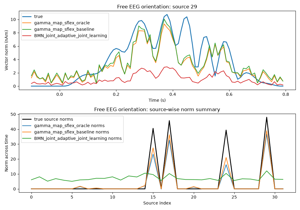
Compare vector-norm summaries for one free-orientation source#
For free orientation, a source has a 3-component time series. A simple scalar summary is the Euclidean norm across orientation components.
free_source_idx = int(np.atleast_1d(active_free)[0])
true_free_component_norm = np.linalg.norm(x_true_free, axis=1)

fig, axes = plt.subplots(2, 1, figsize=(10, 7), sharex=False)
axes[0].plot(times, true_free_component_norm[free_source_idx], label="true", linewidth=2)
for name, result in free_solver_outputs.items():
    est_norm = np.linalg.norm(result["posterior_mean_reshaped"], axis=1)
    axes[0].plot(times, est_norm[free_source_idx], label=name)
axes[0].set(
    xlabel="Time (s)",
    ylabel="Vector norm (nAm)",
    title=f"Free EEG orientation: source {free_source_idx}",
)
axes[0].legend(loc="best")

axes[1].plot(
    np.arange(n_sources),
    np.linalg.norm(true_free_component_norm, axis=1),
    label="true source norms",
    linewidth=2,
    color="black",
)
for name, result in free_solver_outputs.items():
    est_norm = np.linalg.norm(result["posterior_mean_reshaped"], axis=1)
    axes[1].plot(np.arange(n_sources), np.linalg.norm(est_norm, axis=1), label=f"{name} norms")
axes[1].set(
    xlabel="Source index",
    ylabel="Norm across time",
    title="Free EEG orientation: source-wise norm summary",
)
axes[1].legend(loc="best")
fig.tight_layout()
Summary#
SourceEstimator is the main reconstruction wrapper used in the current
CaliBrain pipeline. It standardizes solver invocation and returns posterior
summaries that later feed uncertainty estimation and calibration.
In practice:
use
oraclewhen the simulated sensor noise is available and you want the matched reference variance;use
baselinewhen the noise level should be estimated from the pre-stimulus sensor segment;use
adaptive_joint_learningwhen the solver should learn a common noise level jointly from the data;compare sparse and dense solver families not only by reconstruction, but also by the posterior covariance they hand to the next stage.
The next tutorial takes these posterior outputs and turns them into the uncertainty representations that are actually calibrated:
Total running time of the script: (0 minutes 0.962 seconds)