02. Solver Families and Uncertainty Behavior

This tutorial explains why dense and sparse Bayesian inverse solvers can show different posterior-uncertainty behavior, and why that distinction matters for uncertainty calibration.

Why solver structure matters

CaliBrain does not only compare source estimates. It also compares the uncertainty summaries produced by different Bayesian inverse solvers.

Two broad solver behaviors are especially important:

• dense shared-variance behavior, represented by BMN-type models;

• sparse source-wise variance behavior, represented by gamma-MAP-type models.

Both can produce posterior means and posterior covariance summaries, but they do not typically produce the same uncertainty geometry or the same calibration behavior.

import matplotlib.pyplot as plt
import numpy as np

Dense versus sparse posterior structure

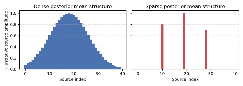
In a dense model, posterior mass is spread broadly across source locations. In a sparse model, many source locations may be strongly suppressed while a smaller subset remains active.

This difference is helpful for localization, but it also affects uncertainty quantification because calibration is built from posterior covariance summaries at the source level.

n_sources = 40
source_idx = np.arange(n_sources)

dense_profile = np.exp(-0.5 * ((source_idx - 18) / 8.0) ** 2)
sparse_profile = np.zeros(n_sources)
sparse_profile[[10, 19, 28]] = [0.8, 1.0, 0.7]

fig, axes = plt.subplots(1, 2, figsize=(8.4, 3.0), sharey=True)
axes[0].bar(source_idx, dense_profile, width=1.0, color="#4c72b0")
axes[0].set_title("Dense posterior mean structure")
axes[1].bar(source_idx, sparse_profile, width=1.0, color="#c44e52")
axes[1].set_title("Sparse posterior mean structure")
for ax in axes:
    ax.set_xlabel("Source index")
    ax.grid(True, axis="y", linestyle="--", alpha=0.35)
axes[0].set_ylabel("Illustrative source amplitude")
fig.tight_layout()

Why sparsity can create uncertainty degeneracy

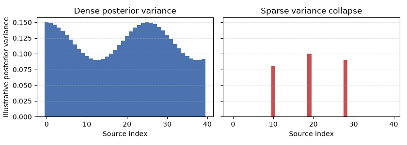
Sparse Bayesian learning can shrink many source-wise variance parameters toward zero. This may improve localization, but it creates a difficulty for uncertainty quantification:

• when local posterior variance collapses to zero,

• the corresponding credible region becomes degenerate or nearly degenerate.

In that case, nominal credible regions can become too small to support meaningful coverage analysis.

dense_variance = 0.12 + 0.03 * np.cos(source_idx / 4.0)
sparse_variance = np.zeros(n_sources)
sparse_variance[[10, 19, 28]] = [0.08, 0.1, 0.09]

fig, axes = plt.subplots(1, 2, figsize=(8.4, 3.0), sharey=True)
axes[0].bar(source_idx, dense_variance, width=1.0, color="#4c72b0")
axes[0].set_title("Dense posterior variance")
axes[1].bar(source_idx, sparse_variance, width=1.0, color="#c44e52")
axes[1].set_title("Sparse variance collapse")
for ax in axes:
    ax.set_xlabel("Source index")
    ax.grid(True, axis="y", linestyle="--", alpha=0.35)
axes[0].set_ylabel("Illustrative posterior variance")
fig.tight_layout()

Why extended support helps

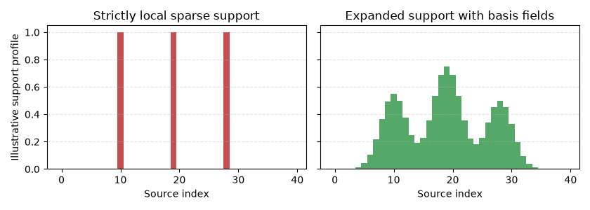
CaliBrain addresses this problem through sparse basis field expansions such as sFLEX. The key idea is that the posterior representation does not remain strictly confined to isolated source locations. Instead, support is expanded through a spatial basis so that local covariance structure remains available for uncertainty analysis.

Conceptually, this changes the uncertainty object from a set of isolated near-zero variance spikes into a smoother source-space covariance structure that can support intervals, ellipses, or ellipsoids.

sparse_support = np.zeros(n_sources)
sparse_support[[10, 19, 28]] = [1.0, 1.0, 1.0]
sflex_support = (
    0.55 * np.exp(-0.5 * ((source_idx - 10) / 2.2) ** 2)
    + 0.75 * np.exp(-0.5 * ((source_idx - 19) / 2.4) ** 2)
    + 0.5 * np.exp(-0.5 * ((source_idx - 28) / 2.2) ** 2)
)

fig, axes = plt.subplots(1, 2, figsize=(8.4, 3.0), sharey=True)
axes[0].bar(source_idx, sparse_support, width=1.0, color="#c44e52")
axes[0].set_title("Strictly local sparse support")
axes[1].bar(source_idx, sflex_support, width=1.0, color="#55a868")
axes[1].set_title("Expanded support with basis fields")
for ax in axes:
    ax.set_xlabel("Source index")
    ax.grid(True, axis="y", linestyle="--", alpha=0.35)
axes[0].set_ylabel("Illustrative support profile")
fig.tight_layout()

Why this affects calibration

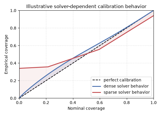
Calibration is based on whether the true source quantity falls inside a credible region constructed from the posterior summary.

Consequently, solver behavior affects calibration in at least two ways:

• through the shape of the posterior mean and covariance;

• through whether the local uncertainty summaries remain non-degenerate.

Dense and sparse models may therefore differ not only in reconstruction accuracy, but also in:

• average posterior uncertainty size,

• underconfidence versus overconfidence,

• robustness of recalibration across settings.

nominal = np.linspace(0.0, 1.0, 200)
dense_curve = np.clip(nominal ** 0.88 + 0.015 * np.sin(2 * np.pi * nominal), 0.0, 1.0)
sparse_curve = np.piecewise(
    nominal,
    [nominal < 0.22, (nominal >= 0.22) & (nominal < 0.6), nominal >= 0.6],
    [
        lambda value: 0.34 + 0.08 * value,
        lambda value: 0.36 + 0.52 * (value - 0.22),
        lambda value: 0.56 + 0.95 * (value - 0.6),
    ],
)
sparse_curve = np.clip(sparse_curve, 0.0, 1.0)

fig, ax = plt.subplots(figsize=(5.6, 4.0))
ax.plot(nominal, nominal, "k--", lw=1.5, label="perfect calibration")
ax.plot(nominal, dense_curve, color="#4c72b0", lw=2.2, label="dense solver behavior")
ax.plot(nominal, sparse_curve, color="#c44e52", lw=2.2, label="sparse solver behavior")
ax.fill_between(nominal, nominal, dense_curve, color="#4c72b0", alpha=0.12)
ax.fill_between(nominal, sparse_curve, nominal, where=sparse_curve <= nominal, color="#c44e52", alpha=0.12)
ax.fill_between(nominal, nominal, sparse_curve, where=sparse_curve > nominal, color="#c44e52", alpha=0.08)
ax.set(
    xlabel="Nominal coverage",
    ylabel="Empirical coverage",
    title="Illustrative solver-dependent calibration behavior",
    xlim=(0, 1),
    ylim=(0, 1),
)
ax.legend(loc="lower right")
ax.grid(True, linestyle="--", alpha=0.35)
fig.tight_layout()

Connection to CaliBrain solvers

In the current toolbox, this distinction appears through the active solver families:

• BMN and BMN_joint represent dense minimum-norm style behavior;

• gamma_map_sflex and gamma_lambda_map_sflex represent sparse gamma-MAP behavior with extended support for uncertainty analysis.

These solver families are compared later at the API level in Source Estimation.

Summary

The main conceptual points are:

1. solver structure changes posterior uncertainty behavior;

2. sparse solvers can create degenerate local uncertainty at pruned sources;

3. extended-support representations help preserve uncertainty summaries that can be used for calibration;

4. calibration differences between solvers are therefore scientifically meaningful, not only numerical side effects.

The next tutorial returns to a minimal runnable example:

• Quick Start