
Note
Go to the end to download the full example code.
10. Orientation and Uncertainty Representations#
This tutorial compares the uncertainty representations used in CaliBrain for fixed orientation, reduced free-orientation MEG, and free-orientation EEG.
The main point is practical: the calibration method depends not only on the solver output, but also on the geometric object used to represent uncertainty.
Scientific question#
CaliBrain supports three main source configurations:
fixed orientation, where each source has one coefficient;
reduced free-orientation MEG, where each source has two coefficients;
free-orientation EEG, where each source has three coefficients.
The uncertainty object changes with that representation:
fixed orientation uses scalar marginal intervals;
reduced free-orientation MEG can use either marginal intervals or full-covariance ellipses;
free-orientation EEG can use either marginal intervals or full-covariance ellipsoids.
In the current workflow, calibration is usually evaluated after temporal aggregation, so this tutorial uses the aggregated coverage routines.
import matplotlib.pyplot as plt
import numpy as np

from calibrain import UncertaintyEstimator


rng = np.random.default_rng(23)
nominal_coverages = np.linspace(0.0, 1.0, 11)
uncertainty = UncertaintyEstimator(nominal_coverages=nominal_coverages)
Fixed orientation: scalar intervals#
For fixed orientation, each source has one value per time point. The uncertainty summary is therefore just a scalar variance per source.
n_sources_fixed = 36
n_times = 90
time = np.linspace(-0.1, 0.7, n_times)

x_true_fixed = np.zeros((n_sources_fixed, n_times))
fixed_active = rng.choice(n_sources_fixed, size=4, replace=False)
fixed_waveform = np.exp(-0.5 * ((time - 0.18) / 0.05) ** 2)
x_true_fixed[fixed_active] = rng.normal(1.0, 0.12, size=(4, 1)) * fixed_waveform

posterior_var_fixed = np.full(n_sources_fixed, 0.055**2)
x_hat_fixed = x_true_fixed + rng.normal(
    scale=np.sqrt(posterior_var_fixed)[:, None],
    size=x_true_fixed.shape,
)

curve_fixed = uncertainty.calibration_curve_intervals_aggregated(
    x_true=x_true_fixed,
    x_hat=x_hat_fixed,
    posterior_var=posterior_var_fixed,
)

print("fixed interval type:", curve_fixed["interval_type"])
print("fixed empirical coverages:", np.round(curve_fixed["empirical_coverages"], 3))
fixed interval type: marginal
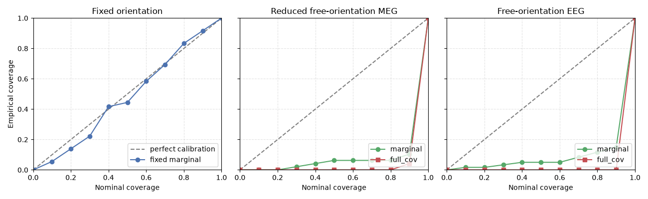
fixed empirical coverages: [0.    0.056 0.139 0.222 0.417 0.444 0.583 0.694 0.833 0.917 1.   ]
Reduced free-orientation MEG: marginal intervals vs full-covariance ellipses#
For reduced free-orientation MEG, each source has two coefficients. CaliBrain can evaluate calibration in two ways:
marginal: component-wise intervals using only the diagonal variances;full_cov: two-dimensional ellipses using the full 2x2 covariance block.
The second representation preserves the within-source covariance geometry.
n_sources_meg = 24
x_true_meg = np.zeros((n_sources_meg, 2, n_times))
meg_active = rng.choice(n_sources_meg, size=4, replace=False)

for source_idx in meg_active:
    amp1, amp2 = rng.normal(loc=[1.0, 0.8], scale=[0.08, 0.08])
    waveform = np.exp(-0.5 * ((time - rng.uniform(0.12, 0.22)) / 0.05) ** 2)
    x_true_meg[source_idx, 0] = amp1 * waveform
    x_true_meg[source_idx, 1] = amp2 * waveform

x_hat_meg = np.zeros_like(x_true_meg)
posterior_cov_meg = np.zeros((n_sources_meg, 2, 2))
V_tan = np.zeros((n_sources_meg, 3, 2))
V_tan[:, 0, 0] = 1.0
V_tan[:, 1, 1] = 1.0
x_true_meg_3d = np.zeros((n_sources_meg, 3, n_times))
x_true_meg_3d[:, :2, :] = x_true_meg

for source_idx in range(n_sources_meg):
    cov_block = np.array([[0.030**2, 0.00045], [0.00045, 0.025**2]])
    mean_error = rng.multivariate_normal(mean=[0.0, 0.0], cov=cov_block)
    x_hat_meg[source_idx, 0] = x_true_meg[source_idx, 0] + mean_error[0]
    x_hat_meg[source_idx, 1] = x_true_meg[source_idx, 1] + mean_error[1]
    posterior_cov_meg[source_idx] = cov_block

curve_meg_marginal = uncertainty.calibration_curve_componentwise_meg_free_aggregated(
    x_true_2d=x_true_meg,
    x_hat_2d=x_hat_meg,
    posterior_uncert_2d=posterior_cov_meg,
)
curve_meg_full = uncertainty.calibration_curve_ellipse_meg_free_aggregated(
    x_true_3d=x_true_meg_3d,
    x_hat_2d=x_hat_meg,
    posterior_cov_2d=posterior_cov_meg,
    V_tan=V_tan,
)

print("MEG marginal empirical coverages:", np.round(curve_meg_marginal["empirical_coverages"], 3))
print("MEG full_cov empirical coverages:", np.round(curve_meg_full["empirical_coverages"], 3))
MEG marginal empirical coverages: [0.    0.    0.    0.021 0.042 0.062 0.062 0.062 0.062 0.104 1.   ]
MEG full_cov empirical coverages: [0.    0.    0.    0.    0.    0.    0.    0.    0.    0.042 1.   ]
Free-orientation EEG: marginal intervals vs full-covariance ellipsoids#
For free-orientation EEG, each source has three coefficients. The same logic applies, but the full-covariance representation is now a three-dimensional ellipsoid instead of a two-dimensional ellipse.
n_sources_eeg = 20
x_true_eeg = np.zeros((n_sources_eeg, 3, n_times))
eeg_active = rng.choice(n_sources_eeg, size=3, replace=False)

for source_idx in eeg_active:
    amps = rng.normal(loc=[1.0, 0.75, 0.55], scale=[0.08, 0.08, 0.08])
    waveform = np.exp(-0.5 * ((time - rng.uniform(0.10, 0.2)) / 0.045) ** 2)
    x_true_eeg[source_idx, 0] = amps[0] * waveform
    x_true_eeg[source_idx, 1] = amps[1] * waveform
    x_true_eeg[source_idx, 2] = amps[2] * waveform

x_hat_eeg = np.zeros_like(x_true_eeg)
posterior_cov_eeg = np.zeros((n_sources_eeg, 3, 3))

for source_idx in range(n_sources_eeg):
    cov_block = np.array(
        [
            [0.032**2, 0.00035, 0.00025],
            [0.00035, 0.028**2, 0.00022],
            [0.00025, 0.00022, 0.024**2],
        ]
    )
    mean_error = rng.multivariate_normal(mean=[0.0, 0.0, 0.0], cov=cov_block)
    x_hat_eeg[source_idx, 0] = x_true_eeg[source_idx, 0] + mean_error[0]
    x_hat_eeg[source_idx, 1] = x_true_eeg[source_idx, 1] + mean_error[1]
    x_hat_eeg[source_idx, 2] = x_true_eeg[source_idx, 2] + mean_error[2]
    posterior_cov_eeg[source_idx] = cov_block

curve_eeg_marginal = uncertainty.calibration_curve_componentwise_eeg_free_aggregated(
    x_true=x_true_eeg,
    x_hat=x_hat_eeg,
    posterior_uncert=posterior_cov_eeg,
)
curve_eeg_full = uncertainty.calibration_curve_ellipsoid_eeg_free_aggregated(
    x_true=x_true_eeg,
    x_hat=x_hat_eeg,
    posterior_cov=posterior_cov_eeg,
)

print("EEG marginal empirical coverages:", np.round(curve_eeg_marginal["empirical_coverages"], 3))
print("EEG full_cov empirical coverages:", np.round(curve_eeg_full["empirical_coverages"], 3))
EEG marginal empirical coverages: [0.    0.017 0.017 0.033 0.05  0.05  0.05  0.083 0.117 0.15  1.   ]
EEG full_cov empirical coverages: [0. 0. 0. 0. 0. 0. 0. 0. 0. 0. 1.]
Compare the calibration curves#
This plot summarizes the main distinction:
fixed orientation has one natural marginal interval representation;
free orientation allows either a marginal representation or a full local covariance representation;
marginalandfull_covare therefore two different calibration diagnostics, not two labels for the same object.
fig, axes = plt.subplots(1, 3, figsize=(13.0, 4.0), sharex=True, sharey=True)

axes[0].plot([0, 1], [0, 1], "--", color="0.5", label="perfect calibration")
axes[0].plot(
    curve_fixed["nominal_coverages"],
    curve_fixed["empirical_coverages"],
    "o-",
    color="#4c72b0",
    label="fixed marginal",
)
axes[0].set_title("Fixed orientation")
axes[0].set_ylabel("Empirical coverage")
axes[0].legend(loc="lower right")

axes[1].plot([0, 1], [0, 1], "--", color="0.5")
axes[1].plot(
    curve_meg_marginal["nominal_coverages"],
    curve_meg_marginal["empirical_coverages"],
    "o-",
    color="#55a868",
    label="marginal",
)
axes[1].plot(
    curve_meg_full["nominal_coverages"],
    curve_meg_full["empirical_coverages"],
    "s-",
    color="#c44e52",
    label="full_cov",
)
axes[1].set_title("Reduced free-orientation MEG")
axes[1].legend(loc="lower right")

axes[2].plot([0, 1], [0, 1], "--", color="0.5")
axes[2].plot(
    curve_eeg_marginal["nominal_coverages"],
    curve_eeg_marginal["empirical_coverages"],
    "o-",
    color="#55a868",
    label="marginal",
)
axes[2].plot(
    curve_eeg_full["nominal_coverages"],
    curve_eeg_full["empirical_coverages"],
    "s-",
    color="#c44e52",
    label="full_cov",
)
axes[2].set_title("Free-orientation EEG")
axes[2].legend(loc="lower right")

for ax in axes:
    ax.set(
        xlabel="Nominal coverage",
        xlim=(0, 1),
        ylim=(0, 1),
    )
    ax.grid(True, linestyle="--", alpha=0.35)

fig.tight_layout()
Practical interpretation#
The calibration workflow should always be read together with the uncertainty representation:
fixed orientation uses scalar source-wise intervals;
free orientation with
marginalchecks component-wise intervals;free orientation with
full_covchecks local ellipses or ellipsoids.
In current CaliBrain workflows, all of these diagnostics are typically
evaluated after averaging over time. The distinction between precal,
post_oracle, post_pooled, post_pooled_mismatch, and
post_fixed then acts on these coverage curves; it does not redefine the
underlying uncertainty geometry.
The next tutorial applies those calibration modes explicitly:
Total running time of the script: (0 minutes 0.274 seconds)