
Note
Go to the end to download the full example code.
03. Quick Start#
This quick start gives the smallest runnable example of CaliBrain’s central object: a pre-calibration empirical coverage curve.
It stays intentionally simple. The goal is to show the core idea in a few lines, then point to the later tutorials that explain each workflow stage in full.
What this quick start shows#
CaliBrain asks whether posterior uncertainty is empirically calibrated.
In the full workflow, that question is answered after:
simulating sources and sensors,
estimating a posterior mean and covariance,
converting that posterior summary into an uncertainty representation,
comparing nominal and empirical coverage.
This quick start jumps directly to step 4 using a lightweight synthetic fixed- orientation example.
import matplotlib.pyplot as plt
import numpy as np

from calibrain import UncertaintyEstimator


RANDOM_SEED = 7
rng = np.random.default_rng(RANDOM_SEED)
Step 1: define a minimal fixed-orientation source example#
The source matrix has shape (n_sources, n_times). Most sources are zero;
a small subset contains ERP-like activity. The full simulation setup is
explained in Source Simulation.
n_sources = 48
n_times = 80
time = np.linspace(-0.2, 0.5, n_times)

x_true = np.zeros((n_sources, n_times))
active_sources = rng.choice(n_sources, size=5, replace=False)
erp_waveform = np.exp(-0.5 * ((time - 0.12) / 0.045) ** 2)
x_true[active_sources] = rng.normal(1.0, 0.2, size=(5, 1)) * erp_waveform
Step 2: define a simple posterior summary#
In real workflows, inverse solvers such as gamma_map_sflex or BMN
produce posterior means and covariance estimates. Those steps are covered in
Source Estimation.
Here we use a simple synthetic posterior summary:
x_hatis the posterior mean;posterior_varis the fixed-orientation marginal variance used by the uncertainty stage.
posterior_var = np.full(n_sources, 0.06**2)
x_hat = x_true + rng.normal(
    loc=0.0,
    scale=np.sqrt(posterior_var)[:, None],
    size=x_true.shape,
)
Step 3: compute the pre-calibration coverage curve#
UncertaintyEstimator builds the uncertainty representation that is used in
the fixed-orientation workflow: aggregated marginal intervals.
The aggregated method averages source time courses over time before checking whether the true source quantity lies inside the interval. The later tutorial Uncertainty Estimation explains this in detail.
nominal_coverages = np.linspace(0.0, 1.0, 11)
uncertainty = UncertaintyEstimator(nominal_coverages=nominal_coverages)
curve = uncertainty.calibration_curve_intervals_aggregated(
    x_true=x_true,
    x_hat=x_hat,
    posterior_var=posterior_var,
)

print("empirical coverages:", np.round(curve["empirical_coverages"], 3))
print("interval type:", curve["interval_type"])
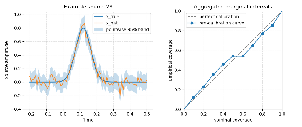
empirical coverages: [0.    0.125 0.229 0.354 0.458 0.542 0.542 0.646 0.771 0.854 1.   ]
interval type: marginal
Step 4: visualize the source example and its calibration curve#
The left panel shows one active source and the posterior mean. The right panel shows the resulting pre-calibration curve.
example_source = int(active_sources[0])

fig, axes = plt.subplots(1, 2, figsize=(10.0, 4.2))

axes[0].plot(time, x_true[example_source], label="x_true", linewidth=2)
axes[0].plot(time, x_hat[example_source], label="x_hat", alpha=0.85)
axes[0].fill_between(
    time,
    x_hat[example_source] - 1.96 * np.sqrt(posterior_var[example_source]),
    x_hat[example_source] + 1.96 * np.sqrt(posterior_var[example_source]),
    alpha=0.25,
    label="pointwise 95% band",
)
axes[0].set(
    xlabel="Time",
    ylabel="Source amplitude",
    title=f"Example source {example_source}",
)
axes[0].legend(loc="best")
axes[0].grid(True, linestyle="--", alpha=0.35)

axes[1].plot([0, 1], [0, 1], "--", color="0.5", label="perfect calibration")
axes[1].plot(
    curve["nominal_coverages"],
    curve["empirical_coverages"],
    "o-",
    label="pre-calibration curve",
)
axes[1].set(
    xlabel="Nominal coverage",
    ylabel="Empirical coverage",
    xlim=(0, 1),
    ylim=(0, 1),
    title="Aggregated marginal intervals",
)
axes[1].set_aspect("equal", adjustable="box")
axes[1].grid(True, linestyle="--", alpha=0.4)
axes[1].legend(loc="best")
fig.tight_layout()
What to read next#
This quick start shows only the smallest runnable coverage example. The later tutorials unpack each stage of the actual workflow:
Total running time of the script: (0 minutes 0.230 seconds)