07. Data Generation

This tutorial explains the high-level DataGenerator class.

It shows how DataGenerator orchestrates benchmark runs across the upstream workflow:

• source simulation;

• leadfield retrieval;

• sensor simulation;

• source estimation;

• run-wise experiment summaries returned as a DataFrame.

Scientific role of DataGenerator

DataGenerator is the benchmark-orchestration layer behind CaliBrain’s upstream workflow. Unlike the lower-level classes, it does not correspond to a single scientific transformation. Instead, it coordinates repeated runs over matched or varying conditions.

Conceptually, its role is:

1. choose a grid of source, sensor, solver, and noise settings;

2. execute one run for each configuration;

3. return run-wise summaries that can later be compared, aggregated, and calibrated.

This tutorial uses a minimal synthetic setup so the orchestration logic can be demonstrated directly.

from tempfile import TemporaryDirectory

import matplotlib.pyplot as plt
import numpy as np
from mne.io.constants import FIFF

from calibrain import DataGenerator, LeadfieldBuilder, SensorSimulator, SourceSimulator, gamma_map_sflex


RANDOM_SEED = 83
tmpdir = TemporaryDirectory()
FIG_DIR = tmpdir.name

# Build a tiny leadfield fixture
# ------------------------------
#
# ``DataGenerator`` expects ``LeadfieldBuilder`` to provide leadfields. In this
# runnable tutorial, we provide a deterministic fixed-orientation EEG leadfield
# through the same high-level builder interface.
#
# Units:
#
# - source amplitudes are in ``nAm``;
# - source coordinates are represented in ``m``;
# - the synthetic EEG leadfield is interpreted as ``µV / nAm``;
# - the resulting simulated EEG sensor signals are therefore in ``µV``.

rng = np.random.default_rng(RANDOM_SEED)
subject = "demo_subject"
n_sensors = 16
n_sources = 32
src_coords = rng.normal(scale=0.04, size=(n_sources, 3))
leadfield = rng.normal(scale=0.03, size=(n_sensors, n_sources))
leadfield /= np.maximum(
    np.linalg.norm(leadfield, axis=0, keepdims=True),
    np.finfo(float).eps,
)
leadfield *= 0.6
q_basis = np.zeros((n_sources, 3, 0), dtype=float)
leadfield_dir = TemporaryDirectory()
np.savez(
    f"{leadfield_dir.name}/{subject}_fixed_leadfield.npz",
    leadfield=leadfield,
    sensor_kind=FIFF.FIFFV_EEG_CH,
    sensor_units=FIFF.FIFF_UNIT_V,
    sensor_unitmult=FIFF.FIFF_UNITM_MU,
    coil_type=FIFF.FIFFV_COIL_EEG,
    src_coords=src_coords,
    Q_basis=q_basis,
)

print("leadfield shape:", leadfield.shape)
print("source coordinates shape:", src_coords.shape)

leadfield shape: (16, 32)
source coordinates shape: (32, 3)

Define a small benchmark grid

DataGenerator is configured from three grids:

• solver_param_grid for estimator hyperparameters;

• data_param_grid for source/sensor-generation settings;

• noise_param_grid for workflow noise handling.

Here we keep them deliberately small. Two alpha_SNR values create two matched runs that differ only in signal-to-noise setting.

erp_config = {
    "tmin": -0.1,
    "tmax": 0.8,
    "stim_onset": 0.0,
    "sfreq": 100,
    "fmin": 2,
    "fmax": 8,
    "amplitude_distribution": {
        "median": 8.0,
        "sigma": 0.15,
        "clip": [2.0, 20.0],
    },
    "random_erp_timing": False,
    "erp_min_length": 20,
}

source_simulator = SourceSimulator(ERP_config=erp_config)
leadfield_builder = LeadfieldBuilder(leadfield_dir=leadfield_dir.name)
sensor_simulator = SensorSimulator()

generator = DataGenerator(
    solver=gamma_map_sflex,
    solver_param_grid={
        "sigma": [0.01],
        "max_iter": [150],
        "tol": [1e-7],
    },
    data_param_grid={
        "subject": [subject],
        "nnz": [4],
        "orientation_type": ["fixed"],
        "alpha_SNR": [0.5, 0.8],
        "sensor_white_noise_std": [0.2],
    },
    noise_param_grid={
        "noise_type": ["oracle"],
    },
    ERP_config=erp_config,
    source_simulator=source_simulator,
    leadfield_builder=leadfield_builder,
    sensor_simulator=sensor_simulator,
    save_posterior_stats=False,
    random_state=RANDOM_SEED,
)

Run the benchmark orchestrator

DataGenerator.run returns a pandas.DataFrame with one row per run. Each row summarizes one experiment in the grid.

results = generator.run(
    nruns=1,
    fig_path=FIG_DIR,
    n_jobs=1,
)

print("result columns:", list(results.columns))
print(results[["global_run_id", "solver", "noise_type", "alpha_SNR", "nnz"]])

2026-07-08 12:14:22 - INFO - [run: 1/1 | config: 1/2 | total: 1/2] gamma_map_sflex | oracle | 4 NNZ | 0.5 SNR
2026-07-08 12:14:22 - INFO - [run: 1/1 | config: 2/2 | total: 2/2] gamma_map_sflex | oracle | 4 NNZ | 0.8 SNR
result columns: ['run_id', 'global_run_id', 'seed', 'solver', 'noise_type', 'max_iter', 'sigma', 'tol', 'alpha_SNR', 'nnz', 'orientation_type', 'sensor_white_noise_std', 'subject', 'sensor_kind', 'coil_type', 'n_sources', 'n_times', 'gamma', 'noise_var', 'active_indices_size']
   global_run_id           solver noise_type  alpha_SNR  nnz
0              1  gamma_map_sflex     oracle        0.5    4
1              2  gamma_map_sflex     oracle        0.8    4

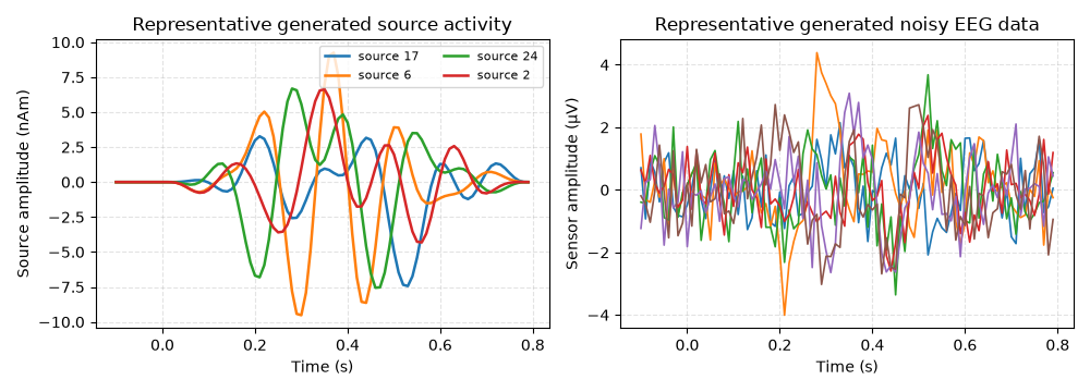
Visualize one representative generated dataset

DataGenerator orchestrates the same source, leadfield, and sensor objects used elsewhere in the toolbox. To make that concrete, we visualize one representative fixed-orientation source realization and its corresponding noisy EEG sensor data under the same tutorial settings.

times = np.arange(
    erp_config["tmin"],
    erp_config["tmax"],
    1.0 / erp_config["sfreq"],
)
x_demo, active_demo = source_simulator.simulate(
    n_sources=n_sources,
    nnz=4,
    orientation_type="fixed",
    seed=RANDOM_SEED,
)
y_clean_demo, y_noisy_demo, _, _ = sensor_simulator.simulate(
    x=x_demo,
    L=leadfield,
    alpha_SNR=0.5,
    sensor_white_noise_std=0.2,
    seed=RANDOM_SEED,
)

fig, axes = plt.subplots(1, 2, figsize=(10.0, 3.6), sharex=True)
for src_idx in active_demo:
    axes[0].plot(times, x_demo[src_idx], lw=1.8, label=f"source {src_idx}")
axes[0].set(
    xlabel="Time (s)",
    ylabel="Source amplitude (nAm)",
    title="Representative generated source activity",
)
axes[0].grid(True, linestyle="--", alpha=0.35)
axes[0].legend(loc="upper right", fontsize=8, ncols=2)

for sensor_idx in range(min(6, y_noisy_demo.shape[0])):
    axes[1].plot(times, y_noisy_demo[sensor_idx], lw=1.2)
axes[1].set(
    xlabel="Time (s)",
    ylabel="Sensor amplitude (µV)",
    title="Representative generated noisy EEG data",
)
axes[1].grid(True, linestyle="--", alpha=0.35)
fig.tight_layout()

What this stage contributes scientifically

At this stage, the key output is not a final calibration result. It is a set of repeated, structured runs that can later be compared across conditions.

In other words, DataGenerator prepares the experimental basis for later questions such as:

• how does calibration change with alpha_SNR?

• how does it change with solver or noise mode?

• how stable are posterior summaries across repeated runs?

Summary

DataGenerator is the high-level orchestration class for the upstream benchmark stage.

In this tutorial it:

• retrieved a leadfield through the standard builder interface;

• simulated source and sensor data;

• ran gamma_map_sflex across a small condition grid;

• returned one row per run for later comparison.

The next workflow stages consume these repeated runs to build uncertainty summaries and calibration analyses.