09. Uncertainty Estimation

This tutorial explains the UncertaintyEstimator class.

It shows how posterior means and posterior covariance matrices are converted into the uncertainty representations that CaliBrain actually calibrates.

It covers:

• fixed-orientation aggregated marginal intervals;

• free-orientation EEG aggregated marginal intervals;

• free-orientation EEG aggregated full_cov ellipsoids;

• pre-calibration empirical coverage curves built from these objects.

Scientific motivation

Source estimation returns posterior means and posterior covariance matrices, but calibration does not operate on those objects directly. UncertaintyEstimator turns them into the uncertainty representations that define the empirical coverage curve.

In the current workflow this means:

• fixed orientation uses scalar posterior_var derived from the diagonal of the covariance;

• free-orientation EEG can be evaluated either with component-wise marginal intervals or with local 3D full_cov ellipsoids;

• the default workflow uses temporally aggregated calibration, so means are averaged over time and covariance is scaled by 1 / T.

Calibration modes such as precal or post_oracle do not change these objects. They act later, on the coverage curves computed from them.

import matplotlib.pyplot as plt
import numpy as np
from mne.io.constants import FIFF

from calibrain import (
    SensorSimulator,
    SourceEstimator,
    SourceSimulator,
    UncertaintyEstimator,
    gamma_map_sflex,
)


RANDOM_SEED = 53
INTERVAL_COLOR = "C0"
POSTERIOR_MEAN_COLOR = "C3"

Build a lightweight posterior example

The tutorial is self-contained: simulate source activity, project it to EEG sensors, add noise, reconstruct sources with gamma_map_sflex, then pass the posterior outputs into UncertaintyEstimator.

Units:

• source amplitudes are in nAm;

• source coordinates for sFLEX are in m;

• EEG leadfields are interpreted as µV / nAm;

• sensor signals are therefore in µV;

• aggregated posterior means remain in nAm and aggregated covariances in the corresponding squared source units.

erp_config = {
    "tmin": -0.1,
    "tmax": 0.8,
    "stim_onset": 0.0,
    "sfreq": 100,
    "fmin": 2,
    "fmax": 8,
    "amplitude_distribution": {
        "median": 8.0,
        "sigma": 0.15,
        "clip": [2.0, 20.0],
    },
    "random_erp_timing": False,
    "erp_min_length": 20,
}

nominal_coverages = np.linspace(0.0, 1.0, 11)
uncertainty_estimator = UncertaintyEstimator(nominal_coverages=nominal_coverages)
source_simulator = SourceSimulator(ERP_config=erp_config)
sensor_simulator = SensorSimulator()

Create small synthetic geometries

To keep the tutorial fast, we generate lightweight synthetic leadfields and, for the free-MEG case, a local tangent basis used to interpret the reduced two-dimensional posterior.

rng = np.random.default_rng(RANDOM_SEED)
n_sensors = 16
n_sources = 32
src_coords = rng.normal(scale=0.04, size=(n_sources, 3))

leadfield_fixed = rng.normal(scale=0.03, size=(n_sensors, n_sources))
leadfield_fixed /= np.maximum(
    np.linalg.norm(leadfield_fixed, axis=0, keepdims=True),
    np.finfo(float).eps,
)
leadfield_fixed *= 0.6

leadfield_free_eeg = rng.normal(scale=0.015, size=(n_sensors, n_sources, 3))
leadfield_free_eeg /= np.maximum(
    np.linalg.norm(leadfield_free_eeg, axis=0, keepdims=True),
    np.finfo(float).eps,
)
leadfield_free_eeg *= 0.4

leadfield_free_meg = rng.normal(scale=0.02, size=(n_sensors, n_sources, 2))
leadfield_free_meg /= np.maximum(
    np.linalg.norm(leadfield_free_meg, axis=0, keepdims=True),
    np.finfo(float).eps,
)
leadfield_free_meg *= 0.5

q_basis_meg = np.empty((n_sources, 3, 2), dtype=float)
for source_idx in range(n_sources):
    q_full, _ = np.linalg.qr(rng.normal(size=(3, 3)))
    q_basis_meg[source_idx] = q_full[:, :2]

sensor_simulator.set_sensor_metadata(
    kind=FIFF.FIFFV_EEG_CH,
    units=FIFF.FIFF_UNIT_V,
    unitmult=FIFF.FIFF_UNITM_MU,
    coil_type=FIFF.FIFFV_COIL_EEG,
)

Fixed orientation: simulate data

We start with the fixed-orientation case because it is the smallest uncertainty representation: one scalar posterior variance per source.

x_true_fixed, active_fixed = source_simulator.simulate(
    n_sources=n_sources,
    nnz=4,
    orientation_type="fixed",
    seed=RANDOM_SEED,
)

y_fixed_clean, y_fixed_noisy, fixed_noise, _ = sensor_simulator.simulate(
    x=x_true_fixed,
    L=leadfield_fixed,
    alpha_SNR=0.7,
    sensor_white_noise_std=0.2,
    seed=RANDOM_SEED,
)
fixed_noise_var = float(np.var(fixed_noise))

Fixed orientation: reconstruct sources

SourceEstimator returns both the posterior mean and the full posterior covariance. UncertaintyEstimator will turn the covariance into the scalar interval representation used for fixed-orientation calibration.

fixed_estimator = SourceEstimator(
    solver=gamma_map_sflex,
    solver_params={"max_iter": 150, "tol": 1e-7, "sigma": 0.01, "src_coords": src_coords},
    noise_var=fixed_noise_var,
    n_orient=1,
)
fixed_estimator.fit(leadfield_fixed, y_fixed_noisy)
fixed_result = fixed_estimator.predict()

posterior_var_fixed = uncertainty_estimator.posterior_variance_from_cov(
    fixed_result["posterior_cov"]
)

print("fixed posterior_mean shape:", fixed_result["posterior_mean"].shape)
print("fixed posterior_cov shape:", fixed_result["posterior_cov"].shape)
print("fixed posterior_var shape:", posterior_var_fixed.shape)

fixed posterior_mean shape: (32, 90)
fixed posterior_cov shape: (32, 32)
fixed posterior_var shape: (32,)

Fixed orientation: build uncertainty objects

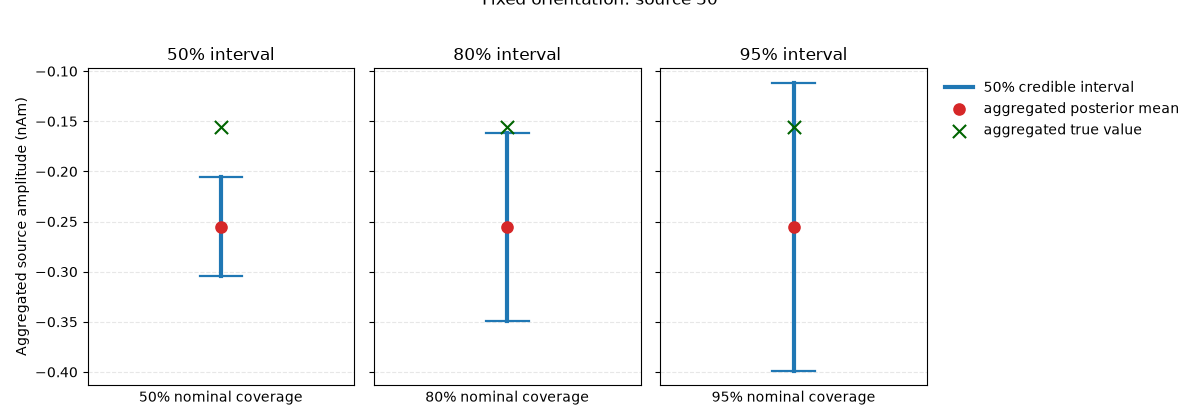
The active workflow uses aggregated calibration. UncertaintyEstimator averages source time courses over time and scales variance by 1 / T before evaluating interval membership.

fixed_membership = uncertainty_estimator.aggregated_interval_membership(
    x_true=x_true_fixed,
    x_hat=fixed_result["posterior_mean"],
    posterior_var=posterior_var_fixed,
    nominal_coverage=0.9,
)
fixed_curve = uncertainty_estimator.calibration_curve_intervals_aggregated(
    x_true=x_true_fixed,
    x_hat=fixed_result["posterior_mean"],
    posterior_var=posterior_var_fixed,
)

print("fixed aggregated empirical coverage at 0.9:", fixed_membership["empirical_coverage"])
print("fixed interval_type:", fixed_curve["interval_type"])

fixed aggregated empirical coverage at 0.9: 1.0
fixed interval_type: marginal

Free EEG: simulate data

For free-orientation EEG, uncertainty estimation can produce two different diagnostics from the same posterior mean and covariance:

• marginal: use only component-wise variances and pool over the three local orientation components;

• full_cov: use each local 3 x 3 covariance block and test coverage with 3D ellipsoids.

This distinction is scientifically important. These are not two labels for the same object; they define different coverage questions.

x_true_free, active_free = source_simulator.simulate(
    n_sources=n_sources,
    nnz=4,
    orientation_type="free",
    coil_type=FIFF.FIFFV_COIL_EEG,
    seed=RANDOM_SEED + 1,
)

y_free_clean, y_free_noisy, free_noise, _ = sensor_simulator.simulate(
    x=x_true_free,
    L=leadfield_free_eeg,
    alpha_SNR=0.7,
    sensor_white_noise_std=0.05,
    seed=RANDOM_SEED + 1,
)
free_noise_var = float(np.var(free_noise))

Free EEG: reconstruct sources

In the free-EEG case, the posterior mean is vector-valued at each source. The covariance can later be interpreted either component-wise or as a full local 3 x 3 block.

free_estimator = SourceEstimator(
    solver=gamma_map_sflex,
    solver_params={"max_iter": 150, "tol": 1e-7, "sigma": 0.01, "src_coords": src_coords},
    noise_var=free_noise_var,
    n_orient=3,
)
free_estimator.fit(leadfield_free_eeg, y_free_noisy)
free_result = free_estimator.predict()

print("free EEG posterior_mean shape:", free_result["posterior_mean"].shape)
print("free EEG posterior_mean_reshaped shape:", free_result["posterior_mean_reshaped"].shape)
print("free EEG posterior_cov shape:", free_result["posterior_cov"].shape)

free EEG posterior_mean shape: (96, 90)
free EEG posterior_mean_reshaped shape: (32, 3, 90)
free EEG posterior_cov shape: (96, 96)

Inspect simulated and reconstructed time series

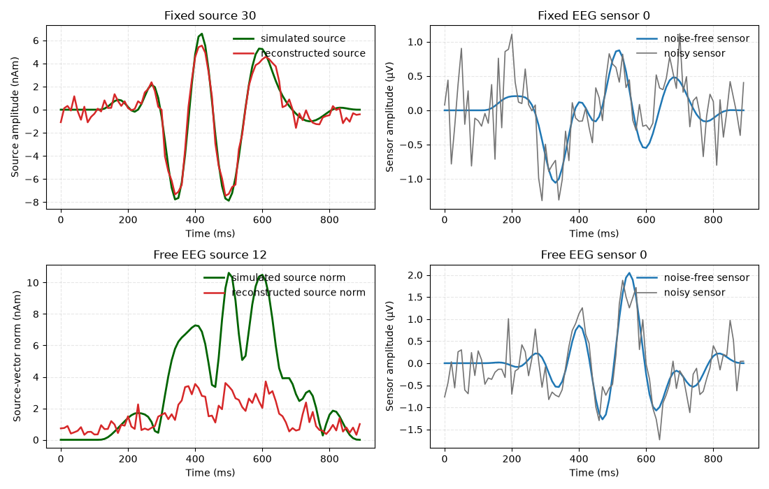
The source panels compare simulated and reconstructed activity. The sensor panels compare the clean forward projection with the noisy observation that is actually passed to the inverse solver.

time_ms = 1e3 * np.arange(x_true_fixed.shape[1]) / erp_config["sfreq"]
fixed_source_idx_ts = int(active_fixed[0])
fixed_sensor_idx_ts = 0
free_source_idx_ts = int(active_free[0])
free_sensor_idx_ts = 0
free_true_norm = np.linalg.norm(x_true_free[free_source_idx_ts], axis=0)
free_recon_norm = np.linalg.norm(
    free_result["posterior_mean_reshaped"][free_source_idx_ts],
    axis=0,
)

fig, axes = plt.subplots(2, 2, figsize=(11.0, 7.0))

axes[0, 0].plot(
    time_ms,
    x_true_fixed[fixed_source_idx_ts],
    color="darkgreen",
    linewidth=2.0,
    label="simulated source",
)
axes[0, 0].plot(
    time_ms,
    fixed_result["posterior_mean"][fixed_source_idx_ts],
    color=POSTERIOR_MEAN_COLOR,
    linewidth=1.8,
    label="reconstructed source",
)
axes[0, 0].set(
    xlabel="Time (ms)",
    ylabel="Source amplitude (nAm)",
    title=f"Fixed source {fixed_source_idx_ts}",
)
axes[0, 0].grid(True, linestyle="--", alpha=0.3)
axes[0, 0].legend(loc="upper right", frameon=False)

axes[0, 1].plot(
    time_ms,
    y_fixed_clean[fixed_sensor_idx_ts],
    color=INTERVAL_COLOR,
    linewidth=1.8,
    label="noise-free sensor",
)
axes[0, 1].plot(
    time_ms,
    y_fixed_noisy[fixed_sensor_idx_ts],
    color="0.45",
    linewidth=1.2,
    label="noisy sensor",
)
axes[0, 1].set(
    xlabel="Time (ms)",
    ylabel="Sensor amplitude (µV)",
    title=f"Fixed EEG sensor {fixed_sensor_idx_ts}",
)
axes[0, 1].grid(True, linestyle="--", alpha=0.3)
axes[0, 1].legend(loc="upper right", frameon=False)

axes[1, 0].plot(
    time_ms,
    free_true_norm,
    color="darkgreen",
    linewidth=2.0,
    label="simulated source norm",
)
axes[1, 0].plot(
    time_ms,
    free_recon_norm,
    color=POSTERIOR_MEAN_COLOR,
    linewidth=1.8,
    label="reconstructed source norm",
)
axes[1, 0].set(
    xlabel="Time (ms)",
    ylabel="Source-vector norm (nAm)",
    title=f"Free EEG source {free_source_idx_ts}",
)
axes[1, 0].grid(True, linestyle="--", alpha=0.3)
axes[1, 0].legend(loc="upper right", frameon=False)

axes[1, 1].plot(
    time_ms,
    y_free_clean[free_sensor_idx_ts],
    color=INTERVAL_COLOR,
    linewidth=1.8,
    label="noise-free sensor",
)
axes[1, 1].plot(
    time_ms,
    y_free_noisy[free_sensor_idx_ts],
    color="0.45",
    linewidth=1.2,
    label="noisy sensor",
)
axes[1, 1].set(
    xlabel="Time (ms)",
    ylabel="Sensor amplitude (µV)",
    title=f"Free EEG sensor {free_sensor_idx_ts}",
)
axes[1, 1].grid(True, linestyle="--", alpha=0.3)
axes[1, 1].legend(loc="upper right", frameon=False)

fig.tight_layout()

Free EEG: build uncertainty objects

marginal works with the same full covariance input, but uses only its diagonal entries source-by-source. full_cov uses the full local 3D blocks.

free_curve_marginal = uncertainty_estimator.calibration_curve_componentwise_eeg_free_aggregated(
    x_true=x_true_free,
    x_hat=free_result["posterior_mean_reshaped"],
    posterior_uncert=free_result["posterior_cov"],
)
free_curve_full_cov = uncertainty_estimator.calibration_curve_ellipsoid_eeg_free_aggregated(
    x_true=x_true_free,
    x_hat=free_result["posterior_mean_reshaped"],
    posterior_cov=free_result["posterior_cov"],
)

free_membership_marginal = uncertainty_estimator.aggregated_componentwise_interval_membership_free(
    x_true=x_true_free,
    x_hat=free_result["posterior_mean_reshaped"],
    posterior_uncert=free_result["posterior_cov"],
    nominal_coverage=0.9,
    n_orient=3,
)
free_membership_full_cov = uncertainty_estimator.aggregated_ellipsoid_membership_eeg_free(
    x_true=x_true_free,
    x_hat=free_result["posterior_mean_reshaped"],
    posterior_cov=free_result["posterior_cov"],
    nominal_coverage=0.9,
)

print("free marginal interval_type:", free_curve_marginal["interval_type"])
print("free full_cov interval_type:", free_curve_full_cov["interval_type"])
print("free marginal empirical coverage at 0.9:", free_membership_marginal["empirical_coverage"])
print("free full_cov empirical coverage at 0.9:", free_membership_full_cov["empirical_coverage"])

free marginal interval_type: marginal
free full_cov interval_type: full_cov
free marginal empirical coverage at 0.9: 0.9791666666666666
free full_cov empirical coverage at 0.9: 1.0

Free MEG: simulate data

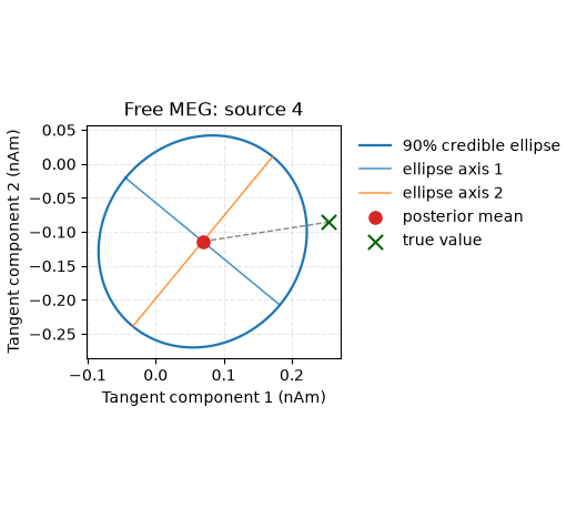
For free-orientation MEG, the posterior lives in a reduced two-dimensional tangential subspace. The uncertainty object is therefore a credible ellipse in that local plane rather than three separate marginal intervals.

x_true_meg_reduced, active_meg = source_simulator.simulate(
    n_sources=n_sources,
    nnz=4,
    orientation_type="free",
    coil_type=FIFF.FIFFV_COIL_VV_MAG_T1,
    seed=RANDOM_SEED + 2,
)
x_true_meg_3d = np.einsum("nck,nkt->nct", q_basis_meg, x_true_meg_reduced)

y_meg_clean, y_meg_noisy, meg_noise, _ = sensor_simulator.simulate(
    x=x_true_meg_reduced,
    L=leadfield_free_meg,
    alpha_SNR=0.7,
    sensor_white_noise_std=0.08,
    seed=RANDOM_SEED + 2,
)
meg_noise_var = float(np.var(meg_noise))

Free MEG: reconstruct sources

Here the posterior mean already lives in the reduced two-dimensional tangent plane. To compare it with the simulated three-dimensional truth, we pass the tangent basis into the uncertainty routines.

meg_estimator = SourceEstimator(
    solver=gamma_map_sflex,
    solver_params={"max_iter": 150, "tol": 1e-7, "sigma": 0.01, "src_coords": src_coords},
    noise_var=meg_noise_var,
    n_orient=2,
)
meg_estimator.fit(leadfield_free_meg, y_meg_noisy)
meg_result = meg_estimator.predict()

meg_curve = uncertainty_estimator.calibration_curve_ellipse_meg_free_aggregated(
    x_true_3d=x_true_meg_3d,
    x_hat_2d=meg_result["posterior_mean_reshaped"],
    posterior_cov_2d=meg_result["posterior_cov"],
    V_tan=q_basis_meg,
)
meg_membership = uncertainty_estimator.aggregated_ellipse_membership_meg_free(
    x_true_3d=x_true_meg_3d,
    x_hat_2d=meg_result["posterior_mean_reshaped"],
    posterior_cov_2d=meg_result["posterior_cov"],
    nominal_coverage=0.9,
    V_tan=q_basis_meg,
)

print("free MEG posterior_mean_reshaped shape:", meg_result["posterior_mean_reshaped"].shape)
print("free MEG posterior_cov shape:", meg_result["posterior_cov"].shape)
print("free MEG interval_type:", meg_curve["interval_type"])
print("free MEG empirical coverage at 0.9:", meg_membership["empirical_coverage"])

free MEG posterior_mean_reshaped shape: (32, 2, 90)
free MEG posterior_cov shape: (64, 64)
free MEG interval_type: full_cov
free MEG empirical coverage at 0.9: 0.9375

Select representative sources for visualization

The fixed-orientation object is a scalar credible interval. The free MEG object is a 2D credible ellipse in the tangential plane. The free EEG object is a 3D credible ellipsoid. Showing these objects explicitly helps clarify what the calibration curves are built from.

fixed_source_idx = int(np.atleast_1d(active_fixed)[0])
free_source_idx = int(np.atleast_1d(active_free)[0])
meg_source_idx = int(np.atleast_1d(active_meg)[0])
free_component_var_agg = free_membership_marginal["posterior_var_agg"][free_source_idx]
fixed_membership_50 = uncertainty_estimator.aggregated_interval_membership(
    x_true=x_true_fixed,
    x_hat=fixed_result["posterior_mean"],
    posterior_var=posterior_var_fixed,
    nominal_coverage=0.5,
)
fixed_membership_80 = uncertainty_estimator.aggregated_interval_membership(
    x_true=x_true_fixed,
    x_hat=fixed_result["posterior_mean"],
    posterior_var=posterior_var_fixed,
    nominal_coverage=0.8,
)
fixed_membership_95 = uncertainty_estimator.aggregated_interval_membership(
    x_true=x_true_fixed,
    x_hat=fixed_result["posterior_mean"],
    posterior_var=posterior_var_fixed,
    nominal_coverage=0.95,
)

Visualize the fixed-orientation uncertainty object

We start with the simplest case: one scalar aggregated source quantity and its credible interval. To make the widening with nominal coverage explicit, we show three separate subplots.

y_levels = np.array([0.5, 0.8, 0.95])
ci_lowers = np.array([
    fixed_membership_50["ci_lower"][fixed_source_idx],
    fixed_membership_80["ci_lower"][fixed_source_idx],
    fixed_membership_95["ci_lower"][fixed_source_idx],
])
ci_uppers = np.array([
    fixed_membership_50["ci_upper"][fixed_source_idx],
    fixed_membership_80["ci_upper"][fixed_source_idx],
    fixed_membership_95["ci_upper"][fixed_source_idx],
])
center_fixed = fixed_membership["x_hat_agg"][fixed_source_idx]
truth_fixed = fixed_membership["x_true_agg"][fixed_source_idx]
fig, axes_fixed = plt.subplots(1, 3, figsize=(12.0, 4.2), sharey=True)

for idx, (ax_fixed, level) in enumerate(zip(axes_fixed, y_levels)):
    ax_fixed.plot(
        [0.5, 0.5],
        [ci_lowers[idx], ci_uppers[idx]],
        color=INTERVAL_COLOR,
        linewidth=3.0,
        label=f"{int(100 * level)}% credible interval",
    )
    whisker_halfwidth = 0.08
    ax_fixed.plot(
        [0.5 - whisker_halfwidth, 0.5 + whisker_halfwidth],
        [ci_lowers[idx], ci_lowers[idx]],
        color=INTERVAL_COLOR,
        linewidth=1.6,
    )
    ax_fixed.plot(
        [0.5 - whisker_halfwidth, 0.5 + whisker_halfwidth],
        [ci_uppers[idx], ci_uppers[idx]],
        color=INTERVAL_COLOR,
        linewidth=1.6,
    )
    ax_fixed.scatter(
        0.5,
        center_fixed,
        color=POSTERIOR_MEAN_COLOR,
        s=65,
        label="aggregated posterior mean",
        zorder=3,
    )
    ax_fixed.scatter(
        0.5,
        truth_fixed,
        color="darkgreen",
        marker="x",
        s=90,
        label="aggregated true value",
        zorder=4,
    )
    ax_fixed.set(
        xlabel=f"{int(100 * level)}% nominal coverage",
        xlim=(0.0, 1.0),
        xticks=[],
        title=f"{int(100 * level)}% interval",
    )
    ax_fixed.grid(True, linestyle="--", alpha=0.3)
    if idx == 0:
        ax_fixed.set_ylabel("Aggregated source amplitude (nAm)")

handles_fixed, labels_fixed = axes_fixed[0].get_legend_handles_labels()
axes_fixed[-1].legend(handles_fixed, labels_fixed, loc="upper left", bbox_to_anchor=(1.02, 1.0), frameon=False)
fig.suptitle(f"Fixed orientation: source {fixed_source_idx}", y=1.02)
fig.tight_layout()

Visualize the free-MEG uncertainty object

The ellipse is built from the aggregated local 2 x 2 covariance block in the tangential plane.

fig, ax_meg = plt.subplots(figsize=(5.2, 4.6))

center2 = meg_membership["projected_mean"][meg_source_idx]
truth2 = meg_membership["projected_true"][meg_source_idx]
Sigma2 = meg_membership["cov_blocks"][meg_source_idx]
threshold2 = float(meg_membership["threshold"])
evals2, evecs2 = np.linalg.eigh((Sigma2 + Sigma2.T) / 2.0)
evals2 = np.maximum(evals2, 1e-12)
radii2 = np.sqrt(threshold2 * evals2)
theta = np.linspace(0.0, 2.0 * np.pi, 361)
circle = np.vstack([np.cos(theta), np.sin(theta)])
ellipse = evecs2 @ np.diag(radii2) @ circle
ax_meg.plot(
    center2[0] + ellipse[0],
    center2[1] + ellipse[1],
    color=INTERVAL_COLOR,
    linewidth=1.6,
    label="90% credible ellipse",
)
for axis_idx in range(2):
    axis_vec = evecs2[:, axis_idx] * radii2[axis_idx]
    ax_meg.plot(
        [center2[0] - axis_vec[0], center2[0] + axis_vec[0]],
        [center2[1] - axis_vec[1], center2[1] + axis_vec[1]],
        linewidth=1.1,
        alpha=0.8,
        label=f"ellipse axis {axis_idx + 1}",
    )
ax_meg.scatter(
    center2[0],
    center2[1],
    color=POSTERIOR_MEAN_COLOR,
    s=65,
    label="posterior mean",
    zorder=3,
)
ax_meg.scatter(
    truth2[0],
    truth2[1],
    color="darkgreen",
    marker="x",
    s=90,
    label="true value",
    zorder=4,
)
ax_meg.plot(
    [center2[0], truth2[0]],
    [center2[1], truth2[1]],
    "--",
    color="0.4",
    linewidth=1.0,
    alpha=0.8,
)
ax_meg.set(
    xlabel="Tangent component 1 (nAm)",
    ylabel="Tangent component 2 (nAm)",
    title=f"Free MEG: source {meg_source_idx}",
)
ax_meg.set_aspect("equal", adjustable="box")
ax_meg.grid(True, linestyle="--", alpha=0.3)
handles_meg, labels_meg = ax_meg.get_legend_handles_labels()
seen_meg = set()
filtered_handles_meg = []
filtered_labels_meg = []
for handle, label in zip(handles_meg, labels_meg):
    if label not in seen_meg:
        filtered_handles_meg.append(handle)
        filtered_labels_meg.append(label)
        seen_meg.add(label)
ax_meg.legend(filtered_handles_meg, filtered_labels_meg, loc="upper left", bbox_to_anchor=(1.02, 1.0), frameon=False)
fig.tight_layout()

Visualize the free-EEG uncertainty object

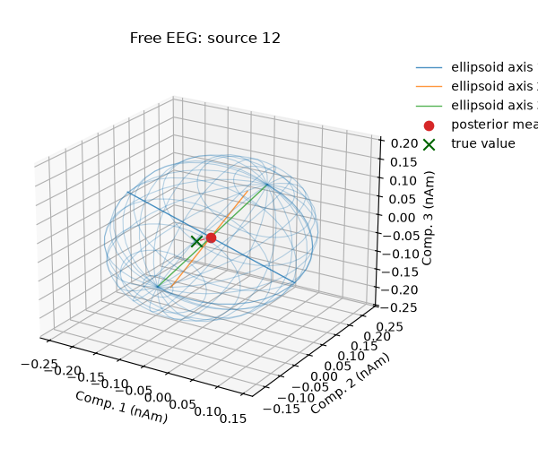
The free-EEG case uses a local 3 x 3 covariance block, so the uncertainty object is a full ellipsoid rather than separate component-wise intervals.

fig = plt.figure(figsize=(6.0, 5.2))
ax_eeg = fig.add_subplot(111, projection="3d")

center3 = free_membership_full_cov["x_hat_agg"][free_source_idx]
truth3 = free_membership_full_cov["x_true_agg"][free_source_idx]
Sigma3 = free_membership_full_cov["cov_blocks"][free_source_idx]
threshold3 = float(free_membership_full_cov["threshold"])
evals3, evecs3 = np.linalg.eigh((Sigma3 + Sigma3.T) / 2.0)
evals3 = np.maximum(evals3, 1e-12)
radii3 = np.sqrt(threshold3 * evals3)
u = np.linspace(0.0, 2.0 * np.pi, 40)
v = np.linspace(0.0, np.pi, 20)
xs = np.outer(np.cos(u), np.sin(v))
ys = np.outer(np.sin(u), np.sin(v))
zs = np.outer(np.ones_like(u), np.cos(v))
sphere = np.stack([xs, ys, zs], axis=0).reshape(3, -1)
ell = (evecs3 @ np.diag(radii3) @ sphere).reshape(3, xs.shape[0], xs.shape[1])
ax_eeg.plot_wireframe(
    center3[0] + ell[0],
    center3[1] + ell[1],
    center3[2] + ell[2],
    rstride=2,
    cstride=2,
    color=INTERVAL_COLOR,
    alpha=0.3,
    linewidth=0.8,
)
for axis_idx in range(3):
    axis_vec = evecs3[:, axis_idx] * radii3[axis_idx]
    ax_eeg.plot(
        [center3[0] - axis_vec[0], center3[0] + axis_vec[0]],
        [center3[1] - axis_vec[1], center3[1] + axis_vec[1]],
        [center3[2] - axis_vec[2], center3[2] + axis_vec[2]],
        linewidth=1.0,
        alpha=0.8,
        label=f"ellipsoid axis {axis_idx + 1}",
    )
ax_eeg.scatter(
    center3[0],
    center3[1],
    center3[2],
    color=POSTERIOR_MEAN_COLOR,
    s=55,
    label="posterior mean",
)
ax_eeg.scatter(
    truth3[0],
    truth3[1],
    truth3[2],
    color="darkgreen",
    marker="x",
    s=80,
    label="true value",
)
ax_eeg.plot(
    [center3[0], truth3[0]],
    [center3[1], truth3[1]],
    [center3[2], truth3[2]],
    "--",
    linewidth=1.0,
    alpha=0.8,
)
ax_eeg.set(
    xlabel="Comp. 1 (nAm)",
    ylabel="Comp. 2 (nAm)",
    zlabel="Comp. 3 (nAm)",
    title=f"Free EEG: source {free_source_idx}",
)
ax_eeg.view_init(elev=22.0, azim=-58.0)
handles_eeg, labels_eeg = ax_eeg.get_legend_handles_labels()
seen_eeg = set()
filtered_handles_eeg = []
filtered_labels_eeg = []
for handle, label in zip(handles_eeg, labels_eeg):
    if label not in seen_eeg:
        filtered_handles_eeg.append(handle)
        filtered_labels_eeg.append(label)
        seen_eeg.add(label)
ax_eeg.legend(filtered_handles_eeg, filtered_labels_eeg, loc="upper left", bbox_to_anchor=(1.02, 1.0), frameon=False)
fig.tight_layout()

Compare the resulting calibration curves

Once the uncertainty objects are defined, calibration curves summarize how often the true aggregated source quantity falls inside them across the full nominal-coverage grid.

fig, axes = plt.subplots(1, 2, figsize=(10, 4.2))
axes[0].plot([0, 1], [0, 1], "--", color="0.5", label="perfect calibration")
axes[0].plot(
    fixed_curve["nominal_coverages"],
    fixed_curve["empirical_coverages"],
    marker="o",
    label="fixed interval",
)
axes[0].plot(
    meg_curve["nominal_coverages"],
    meg_curve["empirical_coverages"],
    marker="s",
    label="free MEG ellipse",
)
axes[0].plot(
    free_curve_full_cov["nominal_coverages"],
    free_curve_full_cov["empirical_coverages"],
    marker="^",
    label="free EEG ellipsoid",
)
axes[0].set(
    xlabel="Nominal coverage",
    ylabel="Empirical coverage",
    title="Dimension-matched uncertainty objects",
)
axes[0].legend(loc="best")

axes[1].plot([0, 1], [0, 1], "--", color="0.5", label="perfect calibration")
axes[1].plot(
    free_curve_marginal["nominal_coverages"],
    free_curve_marginal["empirical_coverages"],
    marker="o",
    label="free marginal",
)
axes[1].plot(
    free_curve_full_cov["nominal_coverages"],
    free_curve_full_cov["empirical_coverages"],
    marker="s",
    label="free full_cov",
)
axes[1].set(
    xlabel="Nominal coverage",
    ylabel="Empirical coverage",
    title="Free EEG: marginal vs full_cov",
)
axes[1].legend(loc="best")
fig.tight_layout()

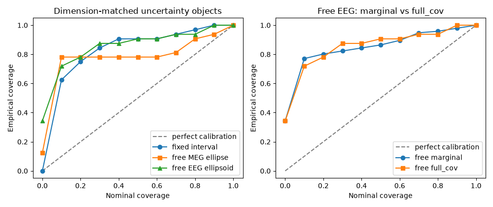
Summary

UncertaintyEstimator is the bridge between posterior covariance and the coverage curves used by calibration.

In the current workflow:

• fixed orientation stores a reduced posterior_var representation;

• free MEG uses a 2D tangential credible ellipse;

• free EEG with marginal uses pooled component-wise variances;

• free EEG with full_cov uses local 3 x 3 covariance blocks;

• aggregated calibration is the default mode, so uncertainty is evaluated on time-averaged predictions.

The next tutorial shows how the calibration stage acts on these curves without changing the underlying uncertainty representation:

• Calibration Methods