Note

Go to the end to download the full example code.

01. Theoretical Foundations#

This tutorial introduces the mathematical foundations used throughout CaliBrain: the orientation-aware forward model, temporally aggregated posterior summaries, source-wise Gaussian marginals, dimension-matched credible regions, empirical coverage, and isotonic recalibration.

Scientific scope#

CaliBrain studies uncertainty calibration for Bayesian M/EEG inverse source imaging. The common question across all workflows is:

what posterior uncertainty object is associated with each source location?
does that uncertainty have the intended empirical coverage?

The framework is built so that fixed orientation, free-orientation MEG, and free-orientation EEG can be treated within one common formulation.

import matplotlib.pyplot as plt
import numpy as np
from sklearn.isotonic import IsotonicRegression

Orientation-aware forward model#

The forward model is

\[y(t) = L x(t) + e(t),\]

with sensor measurement \(y(t)\), leadfield \(L\), source vector \(x(t)\), and noise \(e(t)\).

The local dimension of each source block depends on the orientation model:

fixed orientation: \(d = 1\)
free-orientation MEG: \(d = 2\)
free-orientation EEG: \(d = 3\)

This is why the uncertainty objects differ across settings while the calibration logic remains unified.

Posterior mean and covariance#

The inverse solvers used in CaliBrain return:

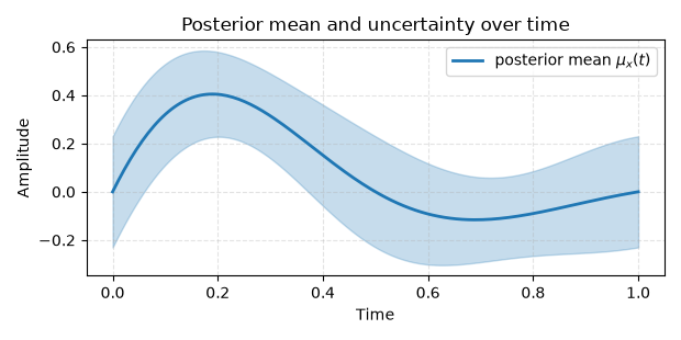
a time-varying posterior mean \(\mu_x(t)\),
a posterior covariance \(\Sigma_x\).

Once hyperparameters are fixed or learned, \(\Sigma_x\) is treated as static across time. This allows uncertainty quantification to be built from a temporally aggregated posterior summary.

time = np.linspace(0, 1, 180)
mu_t = 0.7 * np.sin(2 * np.pi * time) * np.exp(-2.5 * time)
std_t = 0.2 + 0.03 * np.cos(4 * np.pi * time)

fig, ax = plt.subplots(figsize=(6.2, 3.1))
ax.plot(time, mu_t, color="#1f77b4", lw=2, label="posterior mean $\\mu_x(t)$")
ax.fill_between(time, mu_t - std_t, mu_t + std_t, color="#1f77b4", alpha=0.25)
ax.set(xlabel="Time", ylabel="Amplitude", title="Posterior mean and uncertainty over time")
ax.grid(True, linestyle="--", alpha=0.35)
ax.legend(loc="upper right")
fig.tight_layout()

Posterior mean and uncertainty over time

Temporal aggregation#

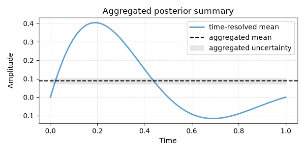
CaliBrain calibration is based on the temporally aggregated source summary

\[\bar{x} = \frac{1}{T} \sum_{t=1}^{T} x(t).\]

Because this is a linear transformation of a Gaussian posterior, the aggregated posterior remains Gaussian:

\[\bar{x} \mid Y \sim \mathcal{N}(\bar{\mu}, \bar{\Sigma}),\]

with

\[\bar{\Sigma} = \frac{1}{T} \Sigma_x.\]

Thus, aggregation preserves the posterior form and scales covariance by \(1/T\).

agg_mean = np.mean(mu_t)
agg_std = np.mean(std_t) / np.sqrt(time.size)

fig, ax = plt.subplots(figsize=(6.2, 3.1))
ax.plot(time, mu_t, color="#1f77b4", lw=2, alpha=0.7, label="time-resolved mean")
ax.axhline(agg_mean, color="black", lw=1.5, ls="--", label="aggregated mean")
ax.fill_between(
    time,
    agg_mean - agg_std,
    agg_mean + agg_std,
    color="gray",
    alpha=0.18,
    label="aggregated uncertainty",
)
ax.set(xlabel="Time", ylabel="Amplitude", title="Aggregated posterior summary")
ax.grid(True, linestyle="--", alpha=0.35)
ax.legend(loc="upper right")
fig.tight_layout()

Local Gaussian marginals#

The full posterior covariance contains dependencies across all source locations and components. For uncertainty quantification, CaliBrain reduces this to source-wise local marginals:

fixed orientation: one scalar variance per source;
free MEG: one local \(2 \\times 2\) covariance block per source;
free EEG: one local \(3 \\times 3\) covariance block per source.

These local blocks are the objects from which credible regions are built.

Dimension-matched credible regions#

For nominal coverage \(c \in (0, 1)\), CaliBrain uses the quadratic-form credible region

\[\mathcal{C}_i(c) = \left\{ z \in \mathbb{R}^{d_i} \;:\; (z - \bar{\mu}_i)^\top \bar{\Sigma}_{ii}^{-1} (z - \bar{\mu}_i) \leq \chi^2_{d_i}(c) \right\}.\]

Here:

\(i\) indexes source locations,
\(d_i \in \{1, 2, 3\}\) is the local source dimension,
\(\bar{\mu}_i\) is the aggregated posterior mean at source \(i\),
\(\bar{\Sigma}_{ii}\) is the local posterior covariance block,
\(\chi^2_{d_i}(c)\) is the \(c\)-quantile of a chi-square distribution with \(d_i\) degrees of freedom.

According to the local dimension \(d_i\), this becomes:

a credible interval for fixed orientation,
a credible ellipse for free MEG,
a credible ellipsoid for free EEG.

Empirical coverage#

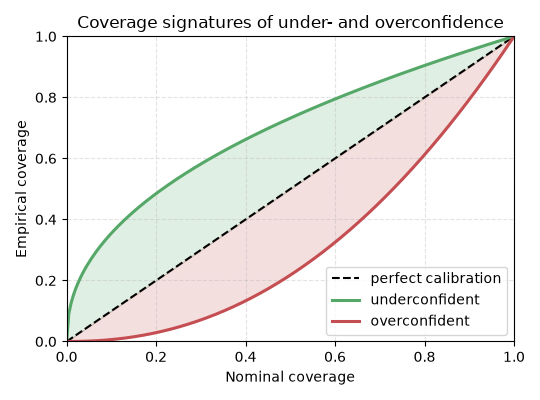
For each nominal coverage level \(c\), CaliBrain checks whether the true aggregated source quantity falls inside the corresponding credible region. Over \(N\) source locations, this gives

\[\hat{c}(c) = \frac{1}{N} \sum_{i=1}^{N} \mathbf{1}\!\left[\bar{x}_i^{\mathrm{true}} \in \mathcal{C}_i(c)\right].\]

Plotting \(\\hat{c}(c)\) against \(c\) produces the calibration curve. Perfect calibration lies on the diagonal.

nominal = np.linspace(0.0, 1.0, 200)
under = nominal ** 0.45
over = nominal ** 2.2

fig, ax = plt.subplots(figsize=(5.4, 4.0))
ax.plot(nominal, nominal, "k--", lw=1.5, label="perfect calibration")
ax.plot(nominal, under, color="#55a868", lw=2.2, label="underconfident")
ax.plot(nominal, over, color="#c44e52", lw=2.2, label="overconfident")
ax.fill_between(nominal, nominal, under, color="#55a868", alpha=0.18)
ax.fill_between(nominal, over, nominal, color="#c44e52", alpha=0.18)
ax.set(xlabel="Nominal coverage", ylabel="Empirical coverage", xlim=(0, 1), ylim=(0, 1))
ax.set_title("Coverage signatures of under- and overconfidence")
ax.grid(True, linestyle="--", alpha=0.35)
ax.legend(loc="lower right")
fig.tight_layout()

Coverage signatures of under- and overconfidence

Isotonic recalibration#

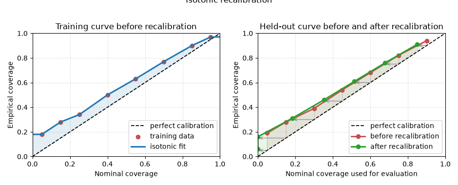
If empirical coverage does not match nominal coverage, CaliBrain applies a monotone recalibration step. The training coverage curve is fitted with isotonic regression, then numerically inverted to obtain recalibrated nominal levels. These corrected levels are evaluated on held-out runs.

This same recalibration mechanism underlies the documented workflow modes. The difference between post_oracle, post_pooled, post_pooled_mismatch, and post_fixed lies in how the training and evaluation runs are chosen.

nominal_grid = np.array([0.05, 0.15, 0.25, 0.4, 0.55, 0.7, 0.85, 0.95])
empirical_raw = np.array([0.18, 0.28, 0.34, 0.5, 0.63, 0.77, 0.9, 0.97])
isotonic = IsotonicRegression(y_min=0.0, y_max=1.0, out_of_bounds="clip")
empirical_fit = isotonic.fit_transform(nominal_grid, empirical_raw)

dense_nominal = np.linspace(0.0, 1.0, 400)
dense_empirical = isotonic.predict(dense_nominal)
evaluation_nominal = np.array([0.05, 0.15, 0.3, 0.45, 0.6, 0.75, 0.9])
evaluation_before = np.array([0.19, 0.28, 0.39, 0.54, 0.68, 0.82, 0.94])
recalibrated_nominal = np.interp(evaluation_nominal, dense_empirical, dense_nominal)
evaluation_after = np.array([0.06, 0.16, 0.31, 0.46, 0.61, 0.76, 0.91])

fig, axes = plt.subplots(1, 2, figsize=(9.4, 3.8))

axes[0].plot([0, 1], [0, 1], "k--", lw=1.3, label="perfect calibration")
axes[0].scatter(nominal_grid, empirical_raw, color="#c44e52", s=35, label="training data")
axes[0].plot(dense_nominal, dense_empirical, color="#1f77b4", lw=2.2, label="isotonic fit")
axes[0].fill_between(dense_nominal, dense_nominal, dense_empirical, color="#1f77b4", alpha=0.12)
axes[0].set(
    xlabel="Nominal coverage",
    ylabel="Empirical coverage",
    xlim=(0, 1),
    ylim=(0, 1),
    title="Training curve before recalibration",
)
axes[0].grid(True, linestyle="--", alpha=0.35)
axes[0].legend(loc="lower right")

axes[1].plot([0, 1], [0, 1], "k--", lw=1.3, label="perfect calibration")
axes[1].plot(
    evaluation_nominal,
    evaluation_before,
    "o-",
    color="#c44e52",
    lw=2.0,
    label="before recalibration",
)
axes[1].plot(
    recalibrated_nominal,
    evaluation_after,
    "o-",
    color="#2ca02c",
    lw=2.2,
    label="after recalibration",
)
for original, corrected, target, before, after in zip(
    evaluation_nominal,
    recalibrated_nominal,
    evaluation_nominal,
    evaluation_before,
    evaluation_after,
):
    axes[1].annotate(
        "",
        xy=(corrected, target),
        xytext=(original, target),
        arrowprops=dict(arrowstyle="->", color="#7f7f7f", lw=1.0, alpha=0.8),
    )
    axes[1].plot([original, original], [target, before], color="#c44e52", alpha=0.25, lw=1.0)
    axes[1].plot([corrected, corrected], [target, after], color="#2ca02c", alpha=0.25, lw=1.0)
axes[1].fill_between(
    evaluation_nominal,
    evaluation_nominal,
    evaluation_before,
    color="#c44e52",
    alpha=0.10,
)
axes[1].fill_between(
    recalibrated_nominal,
    recalibrated_nominal,
    evaluation_after,
    color="#2ca02c",
    alpha=0.10,
)
axes[1].set(
    xlabel="Nominal coverage used for evaluation",
    ylabel="Empirical coverage",
    xlim=(0, 1),
    ylim=(0, 1),
    title="Held-out curve before and after recalibration",
)
axes[1].grid(True, linestyle="--", alpha=0.35)
axes[1].legend(loc="lower right")

fig.suptitle("Isotonic recalibration", y=1.02)
fig.tight_layout()

Isotonic recalibration, Training curve before recalibration, Held-out curve before and after recalibration

Summary#

The theoretical structure behind CaliBrain can be summarized as:

one orientation-aware forward model;
temporally aggregated posterior summaries;
source-wise Gaussian marginals;
dimension-matched credible regions;
empirical coverage curves;
monotone post-hoc recalibration.

The later tutorials move from this mathematical backbone to the concrete implementation:

Solver Families and Uncertainty Behavior motivates why solver structure affects uncertainty summaries;
Quick Start introduces a minimal calibration curve;
Uncertainty estimation builds the uncertainty objects used in practice;
Calibration methods demonstrates recalibration workflows.

Total running time of the script: (0 minutes 0.771 seconds)